Networks of patchy colloids
There will be seen in [this book] demonstrations of those kinds which do not produce as great a certitude as those of geometry, and which even differ much therefrom, since whereas the geometers prove their Propositions by fixed and incontestable Principles, here the Principles are verified by the conclusions to be drawn from them; the nature of these things not allowing of this being done otherwise.
In this chapter, we study networks formed by aggregating patchy particles. Using critical Casimir forces, we assemble divalent and pseudo-trivalent patchy particles by slowly increasing the attractive strength. We compare this near-equilibrium route to a fast quench to high interaction strength and observe that both assembly routes pass through the same equilibrium states, suggesting that the limited valency of particles leads to the formation of an equilibrium gel. The topology of the network is purely set by the equilibrium configuration, independent of its history. Our limited-valency system follows percolation theory remarkably well, and approaches the percolation point with the expected universal exponents. Finally, we show that Flory-Stockmayer theory describes the assembly process well, with a small correction applied for the additional rotational degree of freedom of single monomers.
1. Introduction
Gels are ubiquitous in our daily lives as food and cosmetic products, and of importance in fields ranging from art conservation 1) to Alzheimer research 2) and biomaterials 3). Gels are therefore well studied, but not every aspect of the gelling process is equally well understood. A gel is a dilute microscopic network consisting of interconnecting chains, typically made up of either polymers or colloidal particles. Although the end results of both types of gelation are rather similar, a low-density load-bearing material, their formation process is fundamentally different. A polymer gel is formed by monomers that have a well-defined valency (for instance a mix of monomers with two and three binding sites), undergoing covalent reactions to form a network. Colloidal gels, on the other hand, are typically formed by simple isotropic particles that undergo an arrested phase separation: particles are made strongly attractive (quenched) after which they cluster together and assemble into an out-of-equilibrium network of clustered particles 4).
To describe the formation of a polymer gel, Flory and Stockmayer proposed a series of laws and relations based on graph theory to describe the growth of polymers with a discrete valency into larger and larger networks 5). As it turns out, the principles underlying this chemical process apply to many other fields involving the growth of networks, ranging from the spread rate of forest fires to oil field exploration. The physical basis is given by percolation theory, the study of networks and their properties 6). Unfortunately, due to the fundamentally different formation mechanism, Flory Stockmayer theory (FS) is not applicable to the gelation of colloidal particles as described above. The formation of a colloidal gel is by definition an out-of-equilibrium process, and the properties of the gel are set by the conditions under which gelation takes place 7)8). There is therefore no general theory encompassing the aggregation and structure formation processes in this type of system.
However, simulations and theory have shown that colloidal gels can be formed under equilibrium conditions, given that particles have a limited bonding valency 9)10). Therefore, equilibrium thermodynamics and statistical mechanics can be applied to this system, in contrast to a conventional, out-of-equilibrium colloidal gel, which bonding state is very much dependent on the system’s history. This is an exciting and counterintuitive property, that is of great interest both fundamentally and from an applications’ perspective. Equilibrium gels do not undergo ageing, the slow phase separation process that colloidal gels undergo over time 11), because they are already at the thermodynamically preferred state; the gelling state is now only a function of the thermodynamic parameters of the system 12).
The limited valency required for an equilibrium gel can be achieved using anisotropic colloidal particles decorated with ‘patches’, attractive sites, on their surface. By tuning the size, number, and geometry of these patches, the valency and bonding geometry of these particles can be accurately controlled. This system is very similar to the polymer gels originally considered by Flory-Stockmayer (FS) theory: monomers with well-defined bonding valency cross-link into a network, and such a system can be well described by percolation theory. As such, the assembly of patchy particles into networks has been studied extensively in numerical models, and advanced theoretical predictions based on FS and Wertheim theory have been made13)14)15).
However, experimental confirmation has hardly been obtained, as it has been challenging, if not impossible, to induce particles to undergo sufficiently selective patch-to-patch bonding, especially forming bulk materials. In recent years, the situation has improved with the advancement of patchy-particle synthesis 16), so that experimental studies are becoming available 17)18). Especially work on DNA stars with well-defined valency has been very revealing 19)20). However, these systems are mostly limited to studies of bulk properties, without direct observation of the percolating clusters, making direct comparison of experiment and theory elusive.
In this work, we assemble networks consisting of di- and trivalent colloidal particles, and directly observe the formation of a network using optical microscopy. We elucidate the network properties and formation dynamics of this system by applying classical FS theory. By tuning the patch-to-patch attraction using the critical Casimir force, we explore how the limited valency of the particles leads to the formation of an equilibrium gel. Specifically, we compare a fast quench of the system to a slow near-equilibrium route to percolation, to show that the state of the system is independent of the path. As predicted by FS theory, the bond probability uniquely defines the binding state of the system. As such, FS theory, with small corrections stemming from the quasi-2D nature of the system we consider here, is shown to capture our system remarkably well.
2. Methods
The monomers used to assemble a network are 2- and 4-patch particles with diameters 3.2 μm and 3.7 μm respectively, batch A&B from table 1 of chapter 2. Synthesized by colloidal fusion, the patch sizes are sufficiently small to allow only a single bond between particles per patch to be formed, as follows from chapter 3. Particles are suspended in a binary mixture of water and 2,6-lutidine with lutidine volume fraction \(c_L = 0.25\), with 1 mM \(\mathrm{MgSO_4}\) to increase the bulk-patch contrast, see chapter 2. In this mixture, particles have a gravitational length of approximately \(0.1\) particle diameter, confining particles to the two-dimensional plane of the sample wall. The water-lutidine mixture induces attractive critical Casimir interactions between the particles when close to the critical temperature, \(T_\mathrm{c}\). The distance to this critical temperature, \(\Delta T\), sets the interaction strength between the patches, see chapter 2. In chapter 3 we assembled analogues of alkane molecules using the same particles.
We investigate a particle mixture with a fixed 1:6 mixing ratio of 4- and 2-patch particles with a surface fraction of approximately \(\eta=0.1\). This concentration results in \(S \approx 1700\) particles in our \(\sim\) 240 \(\times\) 240 μm field of view, of which on average, there are \(L \approx\ 240\) 4-patch and \(N \approx\ 1460\) 2-patch particles. There is also a small fraction of ‘dud’ particles $\zeta_\text{dud}: because of synthetic inaccuracies these particles lack patches and are thus not binding and not participating in the network. However, in regular bright-field imaging, dud particles cannot be distinguished from regular particles during experiments. The fraction of dud particles is estimated to be in the order of \(\zeta_\mathrm{dud} = 0.05\).
We adjust the patch-patch attraction by varying the temperature offset from solvent critical temperature between \(\Delta T =\) 0.40 K and \(\Delta T =\) 0.05 K, corresponding to an estimated interaction energy of approximately 2 to \(>15 k_\mathrm{B}T\)(see simulations in chapter 321). Using bright-field microscopy with careful temperature control, we follow the assembly of the network in real-time. Using a modern particle tracking package (TrackPy22)), we locate the centres of all particles, see section 2.3.3. We consider two particles bonded when they are separated by 4.0 μm (approximately \(1.1\) particle diameters) or less, and if this bond persists for at least \(50\) consecutive seconds (5 frames).
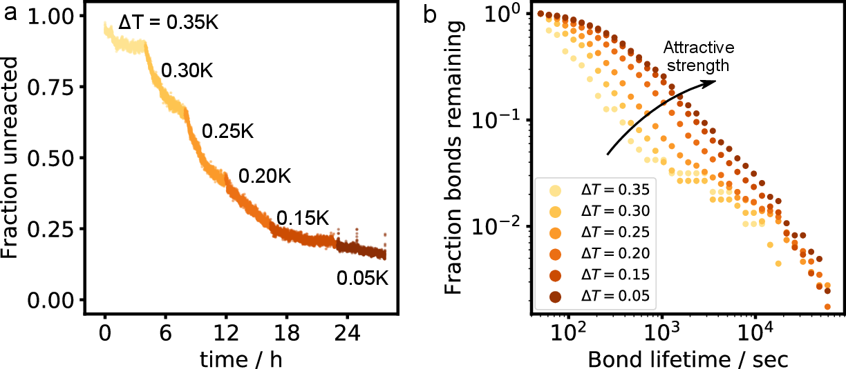
In this work, we explore two different assembly paths: a deep quench to high interaction strength (from \(\Delta T =\) 0.40 K to \(\Delta T =\) 0.05 K in approx. 5 minutes), and a near-equilibrium route, where we increase the interaction strength between particles slowly: starting at \(\Delta T =\) 0.35 K, we wait until we visually confirm the sample is in a steady state (in the order of \(4\)-\(6\) hours), and increase temperature by 0.05 K, where we wait again, followed by another small increment, etc., until we reach \(\Delta T =\) 0.05 K. At low interaction strengths, the bond lifetime is much shorter than the experimental timescale, which leads to a balance of breaking and formation of bonds, see Figure 6b.
3. Results and Discussion
3.1. Hubs & Spokes
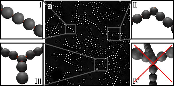
By quickly increasing the interaction strength from 2 to \(>15 k_\text{B}T\) in a quench, patches become strongly attractive, and patch-patch bonds are formed. After about \(4\) hours of assembly, we obtain a network that spans the field of view, see online video 23). Figure 1a shows a snapshot of the assembled structure; the particle network is easily recognized. We observe three types of structural motifs, schematically shown in Figure 1: (I) stiff linear chains consisting of dipatch particles, (II) kinked linear chains consisting of two strands of (I) connected by a tetrapatch particle, and (III) branching points, a central tetrapatch particle connecting three strands of (I). Compared to (I) and (II), structure (III) has a small formation energy penalty because bonding patches point out of plane somewhat due to their tetrahedral arrangement; in chapter 4 we have seen that tetrapatch particles can form 3 bonds in-plane, but at the cost of some energy penalty. Related to that realization is the fact that, despite the \(4\) available bonding sites on a tetrapatch particle, we never observe a tetrapatch particle with \(4\) connected strands in our experiments (Figure 1a-(IV)). Due to the small gravitational height of our particles, such a bonding arrangement will be energetically unfavourable due to the lifting of particles required to form structure (IV).
3.2. Cluster Structure
We hence consider the 4-patch particle as quasi 3-valent, which is essential for a quantitative understanding of our system using Flory-Stockmayer theory. Taking into account the observation that tetrapatch particles have a valency \(f_{N}=3\), the 2- to 4-patch ratio of 6:1 leads to an average valency of \(\left\langle f \right\rangle = \frac{ 1 \cdot 3 + 6 \cdot 2}{6+1} =2\frac{1}{7}\).
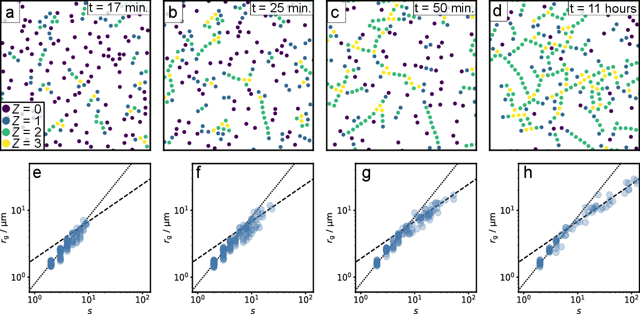
We track particle positions during the assembly process, and show a few representative snapshots in Figure 2a-d. Initially, clusters have a linear geometry and show little branching. As the assembly progresses, structures become increasingly cross-linked. The pseudo-trivalent tetrapatch particles act as hubs, leading to crosslinking between otherwise linear chains. This branching can be quantified by plotting the radius of gyration, \(r_\text{g}\), as a function of the number of particles \(s\) in a cluster, as shown in Figure 2e-h. Initially, the radius grows linearly with the number of particles; resulting in a fractal dimension of \(d_\text{f} = 1\) (dotted line). When structures become larger than approximately \(s=10\) particles, the radius of gyration grows as the power of approximately \(1.8^{-1}\), indicating clusters are now branching, yielding a fractal dimension of \(d_\mathrm{f} = 1.8\) (dashed line) 24). This crossing over to a higher fractal dimension coincides with the behaviour found in simulations on particles with a similarly limited valency, and is close to the percolation universality class value of \(d_\mathrm{f} = 91/48 \), indicating that percolation theory can be used to describe our system 25).
A fractal dimension of \(d_\mathrm{f} = 1.8\) is close to the full coverage of \(2\) dimensions, which is caused by the large density of loops and cross-links in large clusters, clearly visible in the snapshot of Figure 2d. The observation of the formation of loops in larger structures is significant; one of the key assumptions of the FS and Wertheim theories is that bonding loops are non-existent 26)27). Although the classical FS theory does not rely on spatial dimensions, it is known to work well enough for a three-dimensional system, where cross-links are rare 28), but is prone to fail in two-dimensional systems due to the large probability of forming loops 29).
3.3. Cluster Size Evolution - Quench vs Equilibrium
In contrast to the quench route, along which bonds hardly reconfigure, we observe frequent bond-breaking along the near-equilibrium route, especially at lower interaction strength (larger \(\Delta T\)), indicating the system approaches the equilibrium state at each step.
To compare the near-equilibrium route with the fast quench, we follow the second moment of the cluster size distribution, \(C = \sum s^2 N_s / \sum s N_s\), where \(N_s\) is the number of clusters of size \(s\), which is commonly used in percolation theory as measure for the mean cluster size. The growth of the network in the quenched case is shown in Figure 3a. As expected, \(C\) sharply increases initially, stabilizing after approximately 4 hours. The near-equilibrium assembly process shown in Figure 3b on the other hand clearly displays step-wise growth of the network: at each increased interaction strength, the system approaches a new equilibrium cluster size distribution.
We can also follow the progress of the assembly process using the normalized number of bonds in the system, or bond probability, \(p_\mathrm{b}\), defined as
$$ p_\mathrm{b} = \left\langle Z \right\rangle / \left\langle f \right\rangle,$$
where \(\left\langle Z \right\rangle\) is the average number of bonds per particle, and \(\left\langle f \right\rangle\) is the average number of bonding sites per particle. \(\left\langle f \right\rangle\) is simply equal to
$$ \left\langle f \right\rangle = \frac{3N + 2L}{N+L}, $$
with \(N\) 3-valent particles and \(L\) 2-valent particles.
We plot the bond probability and together with the mean cluster size \(C\) in both the quenched and near-equilibrium growth in Figures 3a&b (right axis, hexagons). The bond probability reflects the trend of the mean cluster size \(C\): the quenched system shows a smooth increase to a plateau value, while the near-equilibrium assembly route stabilizes at a constant \(p_\mathrm{b}\) at every intermediate attractive strength. Despite the very different routes to the final state, the eventual bond probability is remarkably similar in both systems: stabilization occurs at \(p_\mathrm{b}\) at \(\Delta T =\) 0.05K.
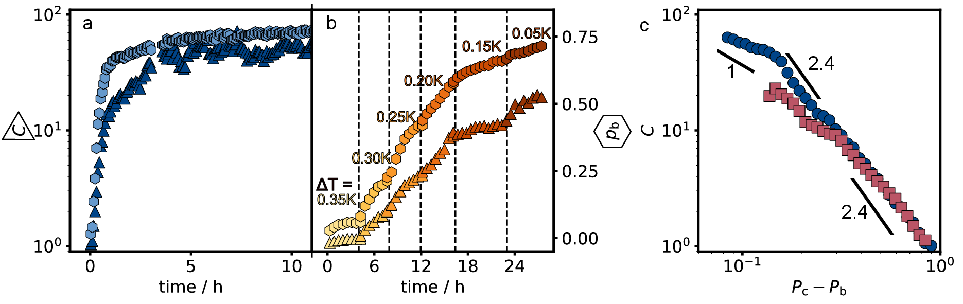
Percolation theory predicts that percolation occurs at the critical bond probability \(p_\mathrm{c} = \frac{1}{\left\langle f \right\rangle - 1} = \frac{1}{2\frac{1}{7}-1} = \frac{7}{8}\) 30). Curiously, both the quenched and near-equilibrium system are very close to percolation at the end of measurements, as illustrated by Figure 2d, however, the observed bond probability of \(p_\mathrm{b} \approx 0.75\) is significantly smaller than \(p_\mathrm{b} = \frac{7}{8} = 0.875\). This difference between predicted and observed percolation threshold is not entirely unexpected: the prevalence of loops in large clusters depresses the bond probability at which percolation takes place. Numerical simulations have encountered similar discrepancies between percolation theory and observation in 2D systems 31).
To check the scaling predictions of percolation theory, we plot the mean cluster size as a function of the distance to the theoretical critical bond probability (\(p_\mathrm{c} - p_\mathrm{b}\)) of both quench and near-equilibrium systems in Figure 3c. The mean cluster size initially increases as a power law with an exponent of 2.4, crossing over to an exponent of approximately 1 in the quench case at \(p_\mathrm{c} - p_\mathrm{b} \approx 0.15\). The divergence approaching the critical point is expected from percolation theory: in a 2D system, \(C\) is expected to diverge with a critical exponent \(\gamma = 43/18 \approx 2.4\), crossing over to 1 close to \(p_\text{c}\) 32), in very good agreement with our observations. Unlike the quench route, the near-equilibrium route does not show a cross-over to a lower exponent, probably because it does not get close enough to the percolation threshold to observe this behaviour. The slight wobble in the data at \(p_\mathrm{c} - p_\mathrm{b} \approx 0.3\) may be associated with the increased likelihood of the presence of rings, influencing the cluster size distribution. Besides this slight deviation, the agreement with percolation theory is striking.
3.4. Cluster Size Distributions
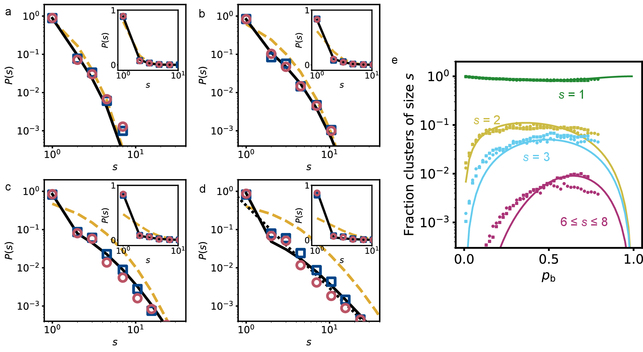
Beside some deviations closer to percolation, the quench and near-equilibrium routes show the same increase in mean cluster size with bond probability, suggesting that the system proceeds through the same aggregation states, uniquely defined by the particle geometry and system bond probability. To further investigate the similarity of both routes, we determine cluster size distributions and plot them for four different bond probabilities and both assembly paths in Figure 4.
Indeed, the experimental cluster size distributions overlap almost perfectly, confirming that we have experimentally realized an equilibrium gel, the physical properties of which do not depend on its history. With increasing bond probability, large clusters become increasingly likely, as seen by the right-shift of the tails in Figures 4a-d. Close to percolation, at \(p_\mathrm{b}=0.73\), the cluster size distribution decreases as a power law with exponent \(\tau = 2.16\), indicated by a black dotted line in Figure 4d. Percolation theory predicts that the number of large clusters of size \(s\) decreases as a power law with two-dimensional universal scaling constant \(\tau = 187/91 \approx 2.05\) close to percolation 33). Our experimentally determined value is only slightly off, indicating a good match with the theory; some deviation is expected due to the inclusion of small clusters in the fit (for which the relation is not expected to hold), the presence of loops in clusters, and possibly because we are not sufficiently close to percolation.
We can further compare our measured cluster size distributions with distributions found from FS theory. FS theory gives the number of clusters \(N_{n,l}\) consisting of \(n\) 3- and \(l\) 2-valent particles as a function of bond probability as 34):
$$ N_{n,l} = N \frac{(1-p_\mathrm{b})^2}{\rho p_\mathrm{b}} [\rho p_\mathrm{b} (1 - p_\mathrm{b})^2]^n [(1-\rho) p_\mathrm{b}]^l \omega_{n,l}.$$
Here, \(\rho = \frac{3 N}{3 N + 2 L}\) is the probability that a randomly chosen patch belongs to an 3-valent particle. The combinatorial term \(\omega_{n,l}\) accounts for the possible conformations of clusters of \(n\) 3-valent and \(l\) 2-valent particles, and is given by eq. [eq:gel-comb]. The cluster size distribution can thus be found for every given bond probability \(p_\mathrm{b}\).
Recent work 35) has shown that in our quasi-2D system, divalent particles exhibiting three-dimensional rotational motion have a lower chance of binding, because patches are not always pointing in plane, but are pointing towards the substrate or are pointing up. In this case, particles will not be able to bind, leading to deviations from FS theory. Luckily, a small correction to FS theory can be made to account for the effect: we define a fraction \(\zeta\) of dipatch particles that are ‘inactive’ and will effectively remain monomers, appearing as clusters of size \(s=1\). We thus calculate \(N_{n,l}\) (eq. [eq:gel-Nnl]), but correct for the number of inactive divalent particles $L_\mathrm{inactive} = \zeta \cdot L$, by subtracting them from the active particles $L_\mathrm{active} = L - L_\mathrm{inactive}$ and adding them to the number of monomers predicted by FS. Since \(zeta\) is hard to accurately estimate, we treat it as a fitting parameter. The full correction is treated comprehensively in section 5.2.
We plot the cluster size distributions obtained from uncorrected (dashed yellow line), and corrected FS theory (solid black line) in Figure 4a-d for four bond probabilities. The experimental data and the predictions from uncorrected FS theory show an increasingly large discrepancy for larger \(p_\mathrm{b}\). The largest difference between experimental data and theory is the number clusters with size \(s=1\): pure FS theory strongly underestimates the number of observed monomers, which is especially clear in the linear insets of Figure 4a-d. The corrected FS theory obtained by fitting the experimental data, with \(= 0.436\) on the other hand agrees exceptionally well with the experimental data. Furthermore, an inactive 2-valent particle fraction of \(= 0.436\) is reasonable based on our particle geometry and theory on a similar system 36).
We further compare the corrected FS model to experimental data over the full range of bond probabilities. In Figure 4e, we plot the fraction of clusters with size \(s=1\), \(s=2\), \(s=3\), and the average of $6\leq s \leq 8$ as a function of bond probability. Again, we note the good overlap between the quenched (squares) and near-equilibrated (dots) datasets. The solid lines indicating the corrected FS predictions are in reasonable agreement with the experimental data. Deviations from FS theory are small, but easily identified due to the logarithmic \(y\)-scale of Figure 5a. At low bond probability, FS predictions underestimate the number of large clusters, probably because \(\zeta\) is not a perfect descriptor of the correction we apply. Additionally, a breakdown of FS theory close to the critical point is expected 37), which we indeed observe.
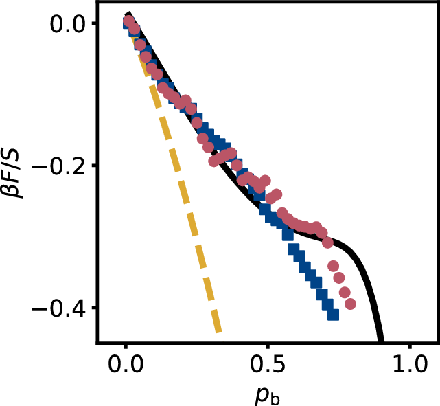
3.5. Free Energy
We further make use of the remarkable properties of an equilibrium gel to directly relate the experimentally determined cluster size distribution to the free energy of the system. By considering our system as a 2-dimensional ideal gas of clusters, the Helmholtz free energy \(F\) can be expressed as
$$ \beta F = N \beta \mu_N + L \beta \mu_L - \sum N_{n,l}, $$
where \(\beta \mu_N = \ln{\frac{N_{1,0}}{A}}\) and \(\beta \mu_L = \ln{\frac{N_{0,1}}{A}}\) are the chemical potentials of the tetra- and dipatch particle respectively with \(A\) the area, and \(\Sigma N_{n,l}\) is the total number of clusters, see section 5.3. All parameters needed to obtain the free energy are related to the cluster size distribution, and thus directly observable in experiment. Therefore, we can easily determine the Helmholtz free energy as a function of bond probability, as shown in Figure 5. Again, the quench and near-equilibrium cases are strikingly comparable: the energies largely overlap. The system energy is calculated from cluster distributions derived from corrected and uncorrected FS theory are in reasonable agreement with experimental results, as we expect based on the similar cluster size distributions shown in Figure 4e. At large bond probabilities, the quenched route appears to describe FS theory predictions better, although more experiments are needed to elucidate this point.
4. Conclusions
Our results convincingly show that this experimental system of divalent and pseudo-trivalent particles form an equilibrium gel. Moreover, experiments show that slowly increasing attractive strength does not lead to a different network architecture as a quick quench to high attractive strengths. While conventional colloidal gel material properties are strongly dependent on the formation history of the gel, the properties of our limited-valency system experiences little to no effect from its exact formation process. We determine several percolation exponents, and note on their remarkable match with predictions from percolation theory. We show that Flory-Stockmayer theory can quantitatively describe our system when we apply a small correction for the extra rotational degree of freedom of monomers for our pseudo-2D geometry. Finally, we show that the free energy of the system can be inferred from the network state directly observed in experiments, made possible due to the equilibrium nature of our gel.
The characteristics of limited-valency networks were predicted through theory and simulations over a decade ago, but experimental conformation has been hard to obtain. In this chapter, we have shown a simple system of patchy particles interacting via critical Casimir forces that display the characteristics predicted by in silica studies. Furthermore, our system is easily studied in real time using optical microscopy, opening the door to facile study of the formed architectures. Our results highlight the exceptional richness of patchy particle assembly: a relatively simple combination of di- and pseudo-trivalent particles can assemble into disordered networks with counterintuitive properties.
5. Appendix
5.1. Temperature-dependent Behaviour
In Figure 3b, we show the evolution of the mean cluster size \(C\) and bond probability \(p_\mathrm{b}\) as a function of time in the near-equilibrium assembly case, which means we see the behaviour as a function of temperature, and thus attractive strength. A few other parameters change as a function of attractive strength that are not explicitly shown in the main text of this chapter. In Figure 6a, we show the evolution of the fraction of unreacted particles (\(N_{s=1}\)). As in Figure 3, we observe a clear stepwise evolution, especially at the lower attractive strengths. There, the faster equilibration takes place because the structures are much more dynamic at low interaction strength. This is examplified in Figure 6b, where we show the bond lifetime at the different temperatures. Clearly, at smaller \(T\) (higher attractive strength), the bond lifetime is much higher, leading to much slower equilibration.
5.2. Correcting Flory-Stockmayer
Flory-Stockmayer theory can be used to predict all network properties as a function of the bond probability, like the number of clusters of a certain composition. In this work, we are interested specifically in the number of clusters \(N_{n,l}\) consisting of \(n\) \(f_{N}\)-valent particles, and \(l\) 2-valent particles; which is equal to 38):
$$ N_{n,l} = N \frac{(1-p_\mathrm{b})^2}{\rho p_\mathrm{b}} [\rho p_\mathrm{b} (1 - p_\mathrm{b})^2]^n [(1-\rho) p_\mathrm{b}]^l \omega_{n,l}, $$
where \(\rho = \frac{f_{N} N}{f_{N} N + 2 L}\) is the probability that a randomly chosen patch belongs to an \(f_{N}\)-valent particle. The combinatorial term \(\omega_{n,l}\) accounts for the possible conformations of clusters of \(n\) \(f//{N}\)-valent and \(l\) 2-valent particles, and is given by:
$$ \omega_{n,l} = f_{N} \frac{ (l + f_{N} n - n) ! }{ l! n! (f_{N} n - 2n + 2)! }. $$
In our system, we have mix of 2- and 3-valent particles, so \(f_{N}=3\), meaning \(\rho = \frac{3 N}{3 N + 2 L}\), as given in the main text, and the combinatorial term simplifies to:
$$ \omega_{n,l} = \frac{ 3 (l + 2 n)! }{ l! n! (n + 2)! }.$$
From our experimental bright-field microscopy images, the 2- and 3-valent particles cannot be distinguished. Therefore, it is convenient to focus on the distribution of total cluster sizes \(s=n+l\), not individual combinations of \(n\) and \(l\). To find the predicted number of clusters of a given size \(s\), we use:
$$ N_s = \sum_{i=0}^{s} N_{i,s-i}, $$
which for a cluster size of \(s=1\) is simply given by \(N_s = N_{0,1} + N_{1,0}\). The cluster size distribution, which is easily determined experimentally, can thus also be found trough FS theory for every given bond probability \(p_\mathrm{b}\).
As mentioned in the main text, recent work 39) has shown that in our quasi-2D system, non-bonded divalent particles exhibiting three-dimensional rotational motion have a lower chance of binding, because patches are not always pointing in plane, but are pointing towards the substrate or are pointing up. In this case, particles will also not be able to bind. Both effects lead to deviations from FS theory. Luckily, small corrections to FS theory can be made to account for the effect: we define a fraction \(\zeta\) of dipatch particles that are ‘inactive’ and will effectively remain monomers, appearing as clusters of size \(s=1\). Practically, we calculate \(N_{n,l}\) (eq. [eq:gel-Nnl]), but corrected for the effective number of active divalent particles, by taking \(\rho' = \frac{3 N}{3 N + 2 L (1-\zeta)}\) Furthermore, we add the inactive particles \(L_\mathrm{inactive} = \zeta \cdot L\) to the number of monomers predicted by FS:
$$ N'_s = $$
$$ \sum_{i=0}^{s} N'\_{i,s-i} + L\_\mathrm{inactive} \text{ , if } s = 1, $$
$$ \sum_{i=0}^{s} N'_{i,s-i} \text{ , if } s >1. $$
Since \(\zeta\) is hard to accurately estimate, we treat it as a fitting parameter.
5.3. Energy of Patchy Networks
If we assume our system is an ideal gas of clusters, we can directly infer the Helmholtz free energy of our system from its cluster size distribution.
The Helmholtz free energy (in units \(k_\mathrm{B} T\)) is given by:
$$ \beta F = \beta G - \beta P A, $$
with \(G\) the Gibbs free energy, and \(P\) and \(A\) the pressure and area respectively. In an ideal gas of clusters, \(P A\) is simply equal to the number of observed clusters:
$$ P A = k_\mathrm{b} T \sum N_{n,l} $$
$$ \beta P A = \sum N_{n,l}. $$
The Gibbs free energy can be expressed in terms of the chemical potential of our di- and tetrapatch particles. At low density, we can approximate the chemical potential of a freely diffusing particle in two dimensions as the logarithm of the particle number density:
$$ \mu^{s=1} = k_\mathrm{b} T \ln \frac{N}{A}, $$
Because of the extraordinary properties of our system, it can be assumed we are always in equilibrium, which means that the chemical potential of e.g. a freely diffusing non-bonded divalent particles must be equal to divalent particles in clusters 40)41), so:
$$ \mu^{s=1}\_L = k_\mathrm{b} T \ln \frac{N_{0,1}}{A} = \mu^{s=2}_L = \mu^{s=3}_L = \dots $$
Therefore, the Gibbs free energy can be obtained in terms of quantities directly observable in our system:
$$ \beta G = N \beta \mu_N + L \beta \mu_L $$
$$ \beta G = N \ln \frac{N_{1,0}}{A} + L \ln \frac{N_{0,1}}{A} $$
with \(N_{1,0}\) the number of monomers that are tetrapatch particles, and \(N_{0,1}\) the number of monomers that are dipatch particles. By combining the above equations, we obtain:
$$ \beta F = N \ln \frac{N_{1,0}}{A} + L \ln \frac{N_{0,1}}{A} - \sum N_{n,l}, $$
which is equivalent to the equation in the main text. The monomer counts \(N_{1,0}\) and \(N_{0,1}\) cannot be determined independently from experiment, since we cannot tell the difference between dipatch and tetrapatch particles from our microscopy images. However, since we know that the corrected FS theory describes our system well, we can use it to determine the number of 2- and 3-valent monomers. The number of monomers is given by
$$ N'\_{s=1} = N_{0,1} + N_{1,0} + L_\mathrm{inactive}, $$
where \(N’_{s=1}\) is the (measured) total number of monomers, \(N_{0,1}\) is the number of 3-valent monomers, and \(N_{1,0} + L_\mathrm{inactive}\) is the number of 2-valent monomers. Using the fitted \(\zeta=0.436\), we can simply determine \(L_\mathrm{inactive} = \zeta L\). Using Flory-Stockmayer, we can determine the ratio between \(N_{1,0}\) and \(N_{0,1}\), which we combine with the observed number of monomers to give the actual di- to trivalent particle ratio:
$$ N_{1,0} = N \frac{(1-p_\mathrm{b})^2}{\rho p_\mathrm{b}} [\rho p_\mathrm{b} (1 - p_\mathrm{b})^2] $$
$$ N_{0,1} = N \frac{(1-p_\mathrm{b})^2}{\rho p_\mathrm{b}} [(1-\rho) p_\mathrm{b}] $$
$$ \frac{N\_{1,0}}{N\_{0,1}} = \frac{\rho}{1-\rho} (1-p_\mathrm{b})^2 $$
$$ N_{1,0} = \frac{N_{1,0}}{N_{0,1}} (S-L_\mathrm{inactive}) $$
$$ N_{0,1} = (S-L_\mathrm{inactive}) - N_{1,0}. $$