Defects of colloidal graphene

Such simple instincts as bees making a beehive could be sufficient to overthrow my whole theory.

Graphene has been under intense scientific interest because of its remarkable optical, mechanical and electronic properties. Its honeycomb structure makes it an archetypical two-dimensional material exhibiting a photonic and phononic band gap with topologically protected states. However, producing large defect-free single-crystal graphene layers remains a great challenge, crucially limiting its applications. Here we assemble colloidal graphene, the analogue of atomic graphene using pseudo-trivalent patchy particles, allowing particle-scale insight into graphene crystal growth and defect dynamics. We directly observe the formation and healing of common defects, like grain boundaries and vacancies. We identify a pentagonal defect motif that is kinetically favoured in the early stages of growth, and acts as seed for more extended defects in the later stages. From the bond saturation and bond angle distortions, we determine the conformational energy of the crystal, and follow its evolution through the energy landscape upon defect rearrangement and healing. These direct observations reveal that the origins of the most common defects lie in the early stages of graphene assembly, where pentagons are kinetically favoured over the equilibrium hexagons of the honeycomb lattice, subsequently stabilized during further growth. Our results open the door to the assembly of complex 2D colloidal materials and investigation of their dynamical, mechanical and optical properties.

Two-dimensional materials have attracted intense scientific interest, both from an application and a fundamental point of view, offering applications from light-weight materials to optoelectronic devices. These materials combine extraordinary mechanical, optical and electronic properties compared to bulk materials ¹⁾²⁾. The most prominent representative, graphene, consists of a monolayer of carbon atoms bonded in a honeycomb lattice. The strong covalent bonds within the honeycomb lattice make the material particularly strong while being light, while the honeycomb structure gives rise to a photonic and phononic band gap ³⁾⁴⁾. Structural defects are known to be central to all of graphene’s properties, enabling among others band-gap tuning in graphene-based electronic devices. However, while defects are introduced unavoidably during growth or added on purpose to tune mechanical and electronic properties, a comprehensive understanding of their formation is missing: because the \(sp^2\)-hybridized carbon atoms can arrange into a variety of polygons and structures, a coherent lattice exists even with defects, and atomic rearrangements can take many paths. Despite recent advances in direct visualization of graphene defects using electron microscopy ⁵⁾⁶⁾, defect kinetics and healing remain poorly understood, and defect-free graphene highly challenging to produce.

Colloids have been used as a model system for crystallization for the better part of a century. Although colloids are several orders of magnitude larger than atoms, their phase behaviour and dynamics is governed by the same thermodynamics principles. Phase behaviour of both atoms and colloids is largely governed by thermal forces, which means we can use colloidal aggregation and crystallization as a simple model for atomic crystallization. This approach has been very successful in the past decades ⁷⁾⁸⁾⁹⁾. One advantage of colloidal systems is that defect formation ¹⁰⁾ and dynamics ¹¹⁾ can be studied directly in real time with single particle resolution, which remains challenging in atomic systems, especially under the harsh high-temperature atomic deposition used for graphene growth. The recently-gained ability to synthesize anisotropic particles ^12)13)14), in particular colloidal particles with attractive patches that provide specific valency and bond angles, has opened a design space for assembling more complex structures such as molecule analogues ^15)16)17).

Simulations and experiment have shown that these colloidal molecules can grow into larger assemblies, yielding rich structures ranging from the kagome lattice to buckyball-like clusters ¹⁸⁾¹⁹⁾. Experimentally realizing these structures however, remains challenging, as they require fine control over specifically coordinated interactions, or purposeful geometric design to block kinetically favoured nonequilibrium routes, as recently shown for the realization of colloidal diamond ²⁰⁾²¹⁾. In contrast to tetrahedrally coordinated diamond, atomic graphene relies on the trivalent coordination of carbon atoms due to their \(sp^2\)-hybridized state. Patchy particles with patches at 120°C angles can mimic these covalent bonds; yet, achieving such valency and controlling these directed bonds on the scale of \(k_T\), the thermal energy, remains challenging, but would open up the assembly of structurally complex 2D materials, and investigation of their structural and mechanical properties.

Here, we assemble colloidal graphene, the colloidal analogue of a monolayer of atomic graphene, and elucidate the kinetic pathways of crystallization and defect formation of this 2D material. We form colloidal graphene using pseudo-trivalent patchy particles adsorbed at a substrate, and directly follow the crystallization, defect formation and healing with great temporal and spatial resolution. Fine control of the patch-patch bond strength allows observation of near-equilibrium assembly in close analogy to high-temperature deposition of atomic graphene. From the number of saturated bonds and the bond strain, we determine the configurational energy of the lattice and follow its evolution during lattice rearrangement and healing. Our results reveal that the most prominent defect motif of colloidal and atomic graphene, a pentagon, is kinetically favoured in the early stages of graphene growth, and acts as seed for extended defects during subsequent growth. These results hint at the importance of the early stages of assembly in generating defect-free graphene.

Figure 1: Colloidal graphene flakes formed from trivalently coordinated particles. (a) Scanning electron microscopy (SEM) image of patchy particle, with patch highlighted in orange. (b) Confocal microscope image of patchy particle, highlighting the fluorescently labelled patches (bright spots). The projected angle between the patches is α=120°. Scale bars in (a) and (b) indicate 1μm. (c) Reconstruction of the surface-bound tetramer patchy particles. One patch is attached to the surface, the remaining three patches available for bonding, making them effectively trivalent. The bonds are tilted slightly out of plane, hence deviating slightly from the ideal in-plane sp^2-like bonding. (d) Confocal microscope image of honeycomb lattice of the pseudo-trivalent particles at ΔT=0.05 °C after 24h of equilibration. Blue and red symbols indicate pentagon and heptagon defects. Scale bar indicates 10μm. Inset: enlarged section with particle centres highlighted in red, showing the honeycomb lattice built out of 6-membered rings. (e, f) Confocal microscope images of the pseudo-trivalent particles at ΔT=0.20 °C (e) and ΔT=0.15 °C (f). With increasing attractive strength, particles assemble into small clusters preferentially containing pentagons (e), which grow into larger structures, favouring hexagons (f). Scale bar indicates 10μm. (g) Fraction of pentagons (blue line), hexagons (black line), and heptagons (red line), and largest cluster size (yellow line) as a function of time. Dashed lines delineate temperature changes. Hexagons grow at the expense of the pentagons.

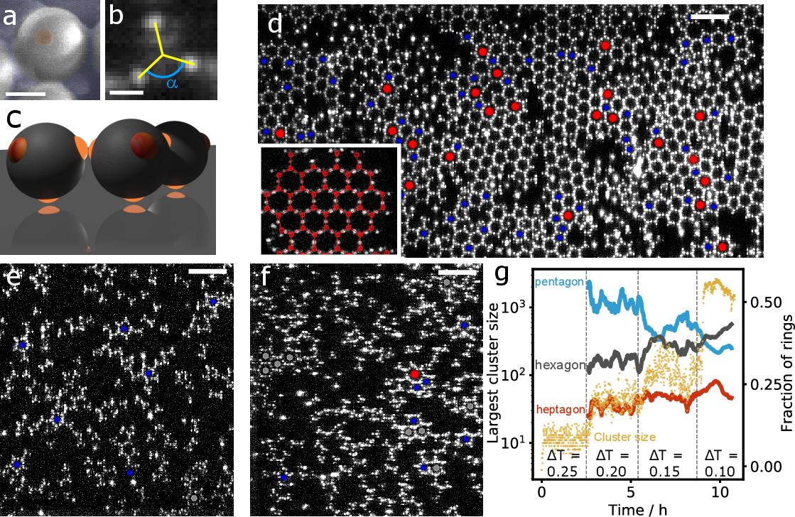
In this chapter, we make use of tetrapatch particles consisting of a polystyrene (PS) bulk and fluorescently labelled 3-(trimethoxysilyl)propyl methacrylate (TPM) patches, synthesized through colloidal fusion as described in chapter 2, see Figure 1a and b ²²⁾. Specifically, we use particle batch C in Table 1, with a diameter of \(\sigma = 2.0\) μm and a patch diameter \(d_\mathrm{p} = 0.2\)μm; the latter is sufficiently small to allow only single patches to bind with each other (see sections 5.3 & 5.4). To induce an effective patch-patch attraction of controllable magnitude, we suspend the particles in a binary solvent close to its critical point. The confinement of solvent fluctuations between the particle surfaces then causes attractive critical Casimir interactions on the order of the thermal energy, \(k_\mathrm{B}T\), tunable by the temperature offset \(\Delta T\) from the solvent critical point, \(T_\mathrm{c}\), see chapter 2.

We use a binary mixture of lutidine and water with lutidine volume fraction \(c_\text{L} = 0.25\) close to the critical volume fraction \(c_\mathrm{L,c} = 0.27\) ²³⁾, and solvent demixing temperature \(T_\mathrm{cx} = 33.95\) °C, and add 1 mM of \(\mathrm{MgSO_4}\) to screen the particles’ electrostatic repulsion and enhance the lutidine adsorption of the hydrophobic patches (see chapter 2). The suspension is injected into a glass capillary with hydrophobically treated walls to which the particles become adsorbed via one of their patches at \(\Delta T \leq\) 0.6 °C. The resulting pseudo-trivalent particles diffuse freely along the surface (see section 5.2), until at \(\Delta T \leq 0.25\) °C, the free patches start attracting each other, as illustrated in Figure 1 (see section 5.6). To observe near-equilibrium assembly, we slowly approach \(T_c\) in steps of 0.05 °C starting from \(\Delta T = 0.25\) °C, leaving the sample to equilibrate for four hours at each step. The resulting slowly increasing patch-patch attraction mimics the slow cooling of atomic systems during high-temperature deposition processes, and ensures a near-equilibrium route to crystallization. We follow the structure and defect formation processes at the particle scale using rapid bright-field and confocal microscope imaging to track both the particles’ centre of mass and fluorescent patches to determine the bond angles with their neighbours (for tracking details, see chapter 2).

The final assembled structure shows large flakes of honeycomb lattice, as shown in Figure 1d. In the lattice, each particle has 3 bonds, at 120° angle with respect to each other, resulting in the repeating 6-membered hexagonal ring motif characteristic of the honeycomb lattice of graphene, as clearly shown in the inset. Indeed, the observation of the honeycomb lattice at our colloidal particle densities is in agreement with simulations of surface-confined trivalent particles predicting the honeycomb lattice for intermediate particle densities ²⁴⁾. Besides the hexagonal honeycomb motif, however, we notice the presence of 5- and 7-membered rings, pentagons and heptagons, often sitting at the boundaries of the honeycomb flakes. The crystal flakes and defects remind of those of atomic graphene grown by chemical or physical vapour deposition. Furthermore, by analogy with atomic deposition, we observe the formation of an amorphous layer when we quench the trivalent particles to high interaction strength (see section 5.5), in line with the amorphous structures observed in low-temperature vapour deposition ²⁵⁾.

To obtain further insight into colloidal graphene growth, we follow the initial stages of assembly at low interaction strength, corresponding to high temperatures in atomic deposition. Surprisingly, many 5-membered rings form initially, as shown in Figure 1e, where small, open pentagon clusters are prevalent (blue dots). As the interaction strength increases, particle clusters grow, and more hexagon motifs, accompanied by heptagon motifs are observed (Figure 1f, grey and red dots, respectively). The dynamic evolution of the different motifs is clearly shown in Figure 1g, where we plot the fraction of pentagons, hexagons, and heptagons, together with the largest cluster size as a function of time. Initially, pentagons are the clear majority, while with increasing attraction, as larger clusters form, the number of hexagons grows at the expense of pentagons until they become the majority and we observe the fully grown flakes in Figure 1d.

Figure 2: Defects in colloidal graphene. Confocal microscope image of a typical grain boundary consisting of pentagons and heptagons. Green dotted boundary separates grains rotated by approx. 17° with respect to each other (left lower inset), which matches observations in atomic graphene (ref. 196). (b) Schematic indicating the compatibility of 5-, 6- and 7-membered rings. Two 6-membered rings and a 5-membered ring leave a 12° angular mismatch, while a combination of one 5-, one 6-, and one 7-membered ring leaves a mismatch of only 3.4°. (c) Confocal microscope image of a divacancy in colloidal graphene. The missing patchy particles are illustrated in grey with orange patches. (d) Confocal microscope image of a polyvacancy. The boundary of the vacancy is indicated with a green line, and the dangling bonds with an orange line segment. In all panels, 6-membered rings are indicated with grey hexagons, 5-membered rings with blue pentagons, and 7-membered rings with red heptagons. The orientation of 6-membered rings is indicated with a black arrow. All images are taken at ΔT=0.05°C. Scale bars in (a), (c) and (d) indicate 5μm.

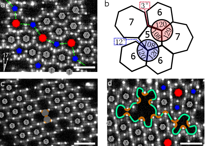
We show examples of the most prominent defect types, grain boundaries and vacancies, in Figure 2. The grain boundary consists of a line of alternating pentagons and heptagons bounding crystalline regions with different orientation above and below, indicated by the green dotted line in Figure 2a. The ‘scar’ of pentagons and heptagons causes a distinct shift in the orientation of the crystal: the honeycomb grains are rotated by approximately 17°. These grain boundaries are very commonly observed in colloidal graphene: the combination of 5- and 7-membered motifs makes them geometrically most compatible with the honeycomb lattice, as shown schematically in Figure 2b. In the ideal lattice, all bond angles are 120°. In contrast, pentagons exhibit internal angles of 108°, incompatible with the honeycomb lattice, making adjacent 6-membered rings unfavourable. Instead, the system typically forms the more favourable combination of alternating pentagons and heptagons, cancelling most of the angular mismatch, see Figure 2b. Hence, the presence of a pentagon facilitates neighbouring heptagons, which in turn promote neighbouring pentagons, stabilizing the grain boundary. Indeed, similar grain boundaries of alternating pentagons and heptagons are found in atomic graphene ²⁶⁾²⁷⁾. Although the details of the inter-atomic attractions are different from those of the colloidal particles, the same geometric argument underlying the typical pentagonal and heptagonal motifs applies.

Vacancies indicate defects, where one or more particles are missing in the honeycomb lattice. An example of a divacancy, where two particles are missing, is shown in Figure 2c, while a bigger poly-vacancy is shown in Figure 2d. In the first case, the surrounding honeycomb lattice is not much perturbed: the crystal structure remains intact, and the orientation of the 6-membered rings does not change. In the second case, the vacancy has a large effect on the surrounding lattice; the lattice is deformed and partly collapsed upon itself.

Vacancies are of interest in atomic graphene, as they can unlock desirable material properties, like catalytic activity and improved electronic properties ²⁸⁾²⁹⁾. However, CVD-grown atomic graphene does not normally show vacancy defects, even though experiments show that vacancies are generated during the early stages of the CVD process ³⁰⁾. Unlike the substrate-adsorbed colloidal particles, carbon atoms can approach vacancies from outside the plane during CVD growth, filling the vacancies with feedstock carbon ³¹⁾. Hence, unlike vacancies in colloidal graphene, vacancies in atomic graphene anneal in the CVD process, and irradiation or chemical treatment is used to induce them. These generated vacancies typically reconfigure to a (slightly) lower-energy structure that contains fewer dangling bonds. For instance, a divacancy can reconfigure into two 5-membered and one 8-membered ring ³²⁾. In contrast, the divacancy in Figure 2c is stable and does not re-configure. We associate this with the more rigid bonds of the short-range critical Casimir interaction potential ³³⁾, making reconfigurations in colloidal graphene unlikely due to high energy barrier (see section 5.8) ^34)35)36).

Figure 3: Origin of defects of colloidal graphene. (a) - (c) Annotated confocal microscope images showing the spontaneous formation of a grain boundary. These images are taken at ΔT=0.10°C, where the honeycomb crystals start forming and are still small. In (a), 2 particles are about to bond, leading to the formation of a 5-membered ring at the red dotted line (blue arrow). In (b), the 5-membered ring has formed, and promotes the formation of a neighbouring 7-membered ring, indicated with the pink arrow. The 7-membered ring in turn promotes the formation of a 5-membered ring next to it, indicated with an orange arrow. In (c), we show the final structure with the blue, pink, and orange arrows indicating the grain-boundary that has grown spontaneously. (d) - (f) Annotated confocal microscope images showing the formation of a grain boundary through the merging of two grains. These images are taken at ΔT=0.05°C. Two larger grains of colloidal graphene approach each other, indicated with green lines and arrows in (d). In (e), the grains have drifted closer together. The red dashed lines indicate where particle bonds will form. The two grains fit together without leaving empty space. In (f) the two grains have merged into one, and alternating 5- and 7-membered rings form their boundary. The rings numbered 1 to 5 are the same in each frame. Scale bars in (a) and (d) indicate 5 μm.

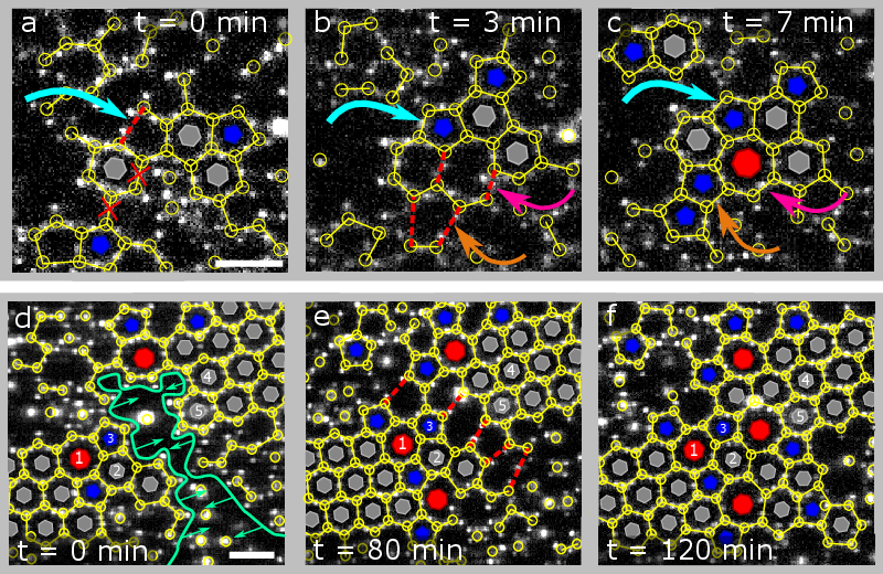
To obtain insight into the origin of the defects, we follow the defect formation process more closely. Pentagons, generated early in the assembly process, can act as nucleation sites for grain boundaries, as shown in Figure 3a-c. The grain boundary grows from a pre-existing pentagon that forms at \(T =\) 0.10 °C (blue arrow in Figure 3a and b), and subsequently ‘catalyses’ the formation of a heptagon, as shown in Figures 3b and c (pink arrow). The heptagon again promotes the formation of a pentagon (orange arrow). Thus, a grain boundary of successive alternating pentagons and heptagons is established after 7 minutes as shown in Figure 3c. We hypothesize that a similar mechanism is effective in atomic graphene. While the role of pentagons in the formation of grain boundaries has not yet been reported for atomic graphene, observations of pentagon formation in early growth of atomic graphene support this possibility ³⁷⁾³⁸⁾. The initial prevalence of pentagons (Figure 1g) favours the formation of the alternating pentagon-heptagon defect, which then remains stable. Yet, this prevalence is surprising, as it is energetically more favourable to form the equilibrium hexagonal motif. Our observations suggest that this effect is of kinetic origin (see section 5.7): a 5-particle ring closes before a sixth particle arrives, and subsequently remains trapped, while continuing to attempt incorporating a sixth particle. A similar kinetically favoured pathway is observed in the assembly of colloidal diamond from tetrahedral particles: 5-membered motifs are kinetically favoured, hindering the formation of the diamond lattice and making it difficult to assemble colloidal diamond ^39)40)41). Similarly, our results on colloidal graphene demonstrate that kinetically favoured pentagons hamper the formation of the equilibrium hexagonal motif, leading to grain boundaries that limit the growth of the honeycomb lattice.

Grain boundaries can also emerge from the merging of crystal grains as shown in Figure 3d-f. The system minimizes the number of dangling bonds by stitching the two crystal islands together, while reconfigurations of the misaligned grains lead to a ‘scar’ of pentagons and heptagons after 120 minutes (see Figure 3f, online video ⁴²⁾, and section 5.9). Similar processes of generating grain boundaries through the merging of crystal grains occur in atomic graphene⁴³⁾⁴⁴⁾.

Figure 4: Defect evolution in colloidal graphene. (a)-(c) Top: Confocal microscope images showing a colloidal graphene polycrystal in its initial configuration (a) and after 4.5 (b) and 9 hours (c) of equilibration at ΔT=0.05 °C. Red and yellow rectangles demarcate regions with static and highly dynamic grain boundaries, respectively. Bottom: Enlarged sections corresponding to the demarcated regions on top. In these sections, 6-membered rings are indicated with grey hexagons, 5-membered rings with blue pentagons, and 7-membered rings with red heptagons. The green solid lines bound poly-vacancies, the orange line segments indicate dangling bonds. Vacancies with 3 dangling bonds are typically monovacancies, vacancies with 4 dangling bonds divacancies. Scale bars in (a) correspond to 5 μm. (d) Total energy per particle computed from dangling bonds and bond bending as a function of time. Red and yellow dots and lines correspond to red and yellow enclosed regions. Dots represent individual frames, solid lines are running averages over one hour (30 data points). The energy curves are shifted with respect to each other for clarity. (e) Energy contributions from dangling bonds and bond bending to the total energy plotted in (d), running averages of 1 hour. Dark colours indicate dangling bond, and light colours bending contributions. (f) Number of pentagons (dashed lines), hexagons (solid lines), and heptagons (dotted lines) present in the two sections as a function of time. The increasing number of hexagons reflecting the closing of these motifs is in line with the decreasing dangling-bond energy in panel (e).

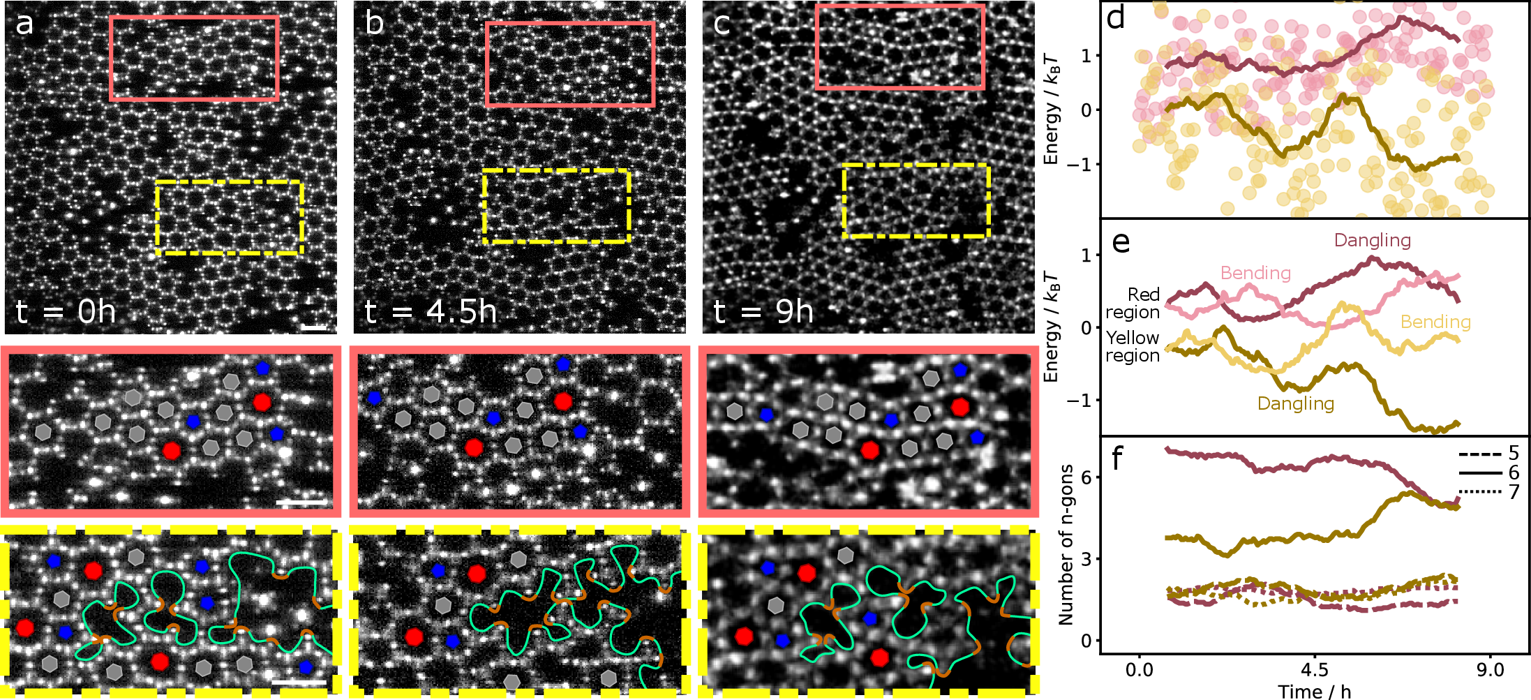
To elucidate the slow reconfiguration of graphene defects in more detail, we follow the graphene polycrystal over a time interval of nine hours. Snapshots of the initial configuration, and after \(4.5\) and \(9\) hours are shown in Figure 4a - c. The red and yellow delineated regions show examples of static and highly dynamic grain boundaries, respectively. The former shows no reorganization: any translation or rotation matches the movement of the entire crystal and the grain boundary is completely frozen. In contrast, the yellow delineated region close to the junction of multiple grains shows significant reconfiguration. The initial monovacancy, divacancy, and larger polyvacancy (Figure 4a) merge into a bigger polyvacancy after \(t =\) 4.5h (Figure 4b), which upon further reconfiguration evolves into a monovacancy, divacancy, and a bigger polyvacancy after \(t = \) 9h (Figure 4c, see video for the full process ⁴⁵⁾). To elucidate the underlying driving force, we follow the total bond energy of the lattice over time. We include two energy contributions: energy costs due to unsaturated bonds, and energy costs due to structural distortions, where we consider only contributions from bond bending. The resulting total energy as a function of time (Figure 4d) reveals an energy landscape with maxima and minima, which clearly decreases for the yellow region, while it remains fairly constant for the red region. The data suggests that the yellow region slowly transitions towards a more favourable lower-energy state, while moving through the energy landscape, unlike the red region that cannot easily lower its energy.

To further elucidate the reconfiguration process, we plot the two energy contributions separately in Figure 4e. Both are of similar order of magnitude, while the dangling bond contribution dominates the total energy drop. Interestingly, bending and dangling-bond contributions show opposite behaviour in the first case, revealing the system’s frustration (closing of bonds leads to lattice distortions and vice versa), while in the dynamic case, the two contributions decrease in parallel, leading to energetically more favourable configurations. Apparently, the interplay of lattice distortion and dangling bond saturation determines the reconfiguration process. This is further corroborated in Figure 4f, where we show the evolution of the number of hexagons (solid lines), pentagons and heptagons (dashed and dotted lines). The increasing number of hexagons accompanying the decreasing bending and dangling bond energy highlights the system’s approach to the energetically most favourable honeycomb lattice, in contrast to the static case. The number of pentagons and heptagons changes only slightly in both cases.

The observed reconfigurations remind of the atomic reconfigurations observed at large holes of graphene using time-resolved high-resolution electron microscopy ⁴⁶⁾, where individual atoms continuously bind and unbind at the hole edges. Our time and particle-resolved observations of colloidal graphene allow detailed insight into the defect dynamics of this important 2D material, highlighting the strong dynamical nature of large vacancies and the corresponding changes in the energy landscape.

Trivalent colloidal particles adsorbed at a substrate form the colloidal analogue of graphene, allowing direct observation of its crystallization and defect dynamics. Fine interaction control opens near-equilibrium crystallization pathways in close analogy to atomic deposition processes of atomic graphene. We find that colloidal graphene defects originate in the early stages of crystallization from pentagonal particle motifs that are kinetically favoured over the equilibrium hexagonal motifs, further stabilized by adjacent heptagonal motifs, together forming stable grain boundaries. These results are consistent with high-resolution electron microscopy observations of atomic graphene, which however are limited to fully grown graphene, and cannot access the initial stages of crystallization. Grain boundaries and extended polyvacancies reconfigure towards lower-energy states by an interplay of dangling-bond saturation and lattice distortions, ultimately increasing the number of hexagons. Strategies for synthesizing large atomic graphene crystals tend to circumvent this issue by either generating as few graphene seeds as possible ⁴⁷⁾, or aligning graphene islands before merging ⁴⁸⁾. While crystallization and defect dynamics in atomic graphene are ultimately governed by quantum mechanics, we expect that in the high-temperature limit studied here, where the quantum-mechanical states become quasi-continuous, our colloidal system provides a good model; yet, differences may arise from the different form of the potential and resulting differences in the bending stiffness of the colloidal and atomic bonds.

The assembly of colloidal graphene demonstrates the increasing control over bottom-up assembly of complex materials. The honeycomb lattice is of specific interest because it is the simplest metamaterial exhibiting photonic and phononic bandgap^49)50)51), and topologically protected states. While achieving the structural complexity of macroscopic mechanical metamaterials remains still a challenge, our results demonstrate that the necessary structural motifs can be assembled using patchy particles, opening the door to microscale mechanical metamaterials ⁵²⁾.

Tetrapatch particles (diameter of 2.0 μm, patch diameter of approx. 0.5 μm, batch C in Table 1 of chapter 2, see sections 5.3 & 5.6) are dispersed in the regular binary solvent of \(25%\) 2,6-lutidine (>99%, Sigma Aldrich) and 75% milliQ water with 1mM \(\mathrm{MgSO_4}\) (>99.5%, Sigma-Aldrich), as described in chapter 2. The particles are washed several times in the water-lutidine mixture. The resulting particle dispersion is injected into a silanized hydrophobic glass capillary and sealed with teflon grease (for full preparation see chapter 2).

Particles are left to sediment to the bottom of the sample at room temperature before measurements. We tilt the sample slightly during sedimentation, so a small density gradient is present in the sample. We then heat the sample to approximately 33.35 °C ($\Delta T \approx 0.6$ °C), which causes one of the particle patches to attach to the sample wall. For heating, we use a well-controlled temperature stage in combination with an objective heating element.

In an experiment, we typically heat a sample to a certain \(T\) below the phase separation temperature of the water-lutidine mixture, inducing critical Casimir attraction between patches. The structures then grow by two-dimensional diffusion in the plane. No mixing is necessary. We investigate the structures as they form using a 100x oil-immersion objective, and image the assembled structures using confocal microscope image stacks, sometimes alternating with bright field images. The particle locations are tracked via the network-based approach described in chapter 2.

Figure 5: Mean square displacement (MSD) of particles bound to the surface. Red circles indicate ΔT=0.60 °C, blue squares ΔT=0.05 °C. The MSD can be fitted using the equation r^2=4D x t^n, where D is the diffusion coefficient, t is the lag time, and n is the exponent. In an ideal system of free diffusion, n=1. The black solid line is a fit of our data, yielding a diffusion coefficient D=0.88 μm^2/s and n=0.95.

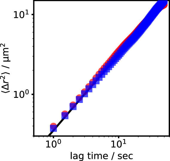
To check the influence of the surface attraction on the mobility of the particles, we determined the mean square displacement of particles at the glass at \(\Delta T =\) 0.05°C and \(\Delta T =\) 0.60°C, see Figure 5. These temperatures correspond to the extreme cases of maximal critical Casimir attraction explored, and minimal Casimir attraction required for the particles to adsorb at the surface. Nevertheless, the mean-square displacement of the particles overlap, suggesting negligible influence of the attraction on the mobility: we observe a power-law behaviour with slope \(\sim 1\), as expected for free diffusion, and with diffusion constant \(D =\) 0.88 μm\(^{2}s^{-1}\). Furthermore, the two different attractions investigated show the same diffusion constant within error bars. Apparently, the stronger attraction of the particles to the wall does not influence the particles’ diffusion through interaction with the wall via hydrodynamic effects or friction.

Figure 6: Particle size distribution. Probability distribution of inter-particle distances between our particles. The orange line indicates a normal distribution with average particle diameter 2.00 μm and a standard deviation of 0.05 μm.

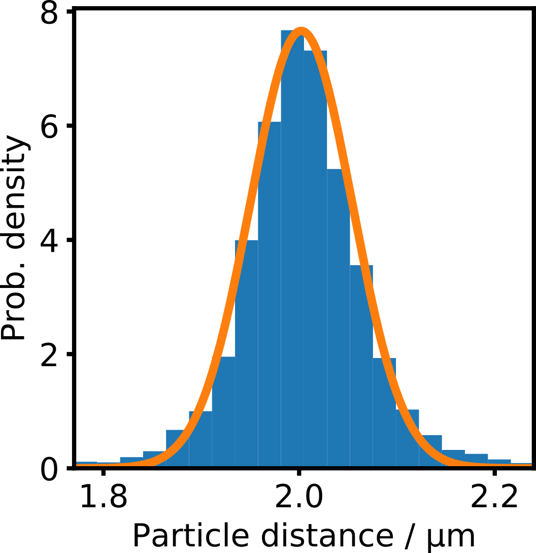
The effective particle diameter can be determined directly from assembly experiments. We determine the inter-particle distances between particles in the honeycomb lattice. In an assembled structure, the centre-to-centre particle distances of bonded tetramer particles should correspond to twice the particle radius plus twice the patch height plus twice the (short) interaction range, as described in chapter 2. The mean of the inter-particle distance distribution at 2.00 μm reflects the effective particle size as estimated from SEM (see Figure 1a), and a standard deviation of \(\sigma =\) 0.05μm.

Figure 7: Assembly of patchy particles. We assemble particles by performing a step-wise temperature ramp: we start at 33.70 °C ΔT=0.25 °C). Every 2.6h, we increase the temperature (equivalent to decreasing ΔT by 0.05°C. (a) Bright field microscopy image of assembled particles after approx. 17 hours, at ΔT=0.05°C. Most particles are part of a small structure. The inset shows that particles are ordered hexagonally. (b) We follow the size of the largest cluster during a temperature ramp. Dashed vertical lines indicate temperature changes. (c) In the same ramp, we track the fraction of rings that are pentagons (blue), hexagons (grey), and heptagons (red) as a function of time. Dots show data for individual frames, and solid lines show the moving average over 10 minutes (20 data points). Initially, there are no/very few rings, but as ΔT becomes smaller, larger structures, including rings are formed. At ΔT=0.20°C, the majority of rings is pentagons. However, with decreasing ΔT, hexagonal rings take over.

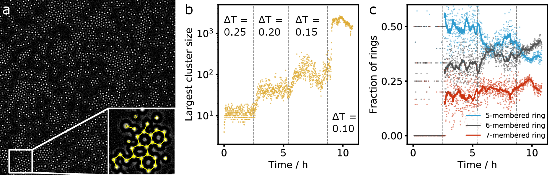
To assemble the particles near-equilibrium, we slowly increase the temperature in steps of 0.05 °C starting from \(\Delta T =\) 0.25 °C, waiting at each temperature for 4 hours. This way, the system has time to adjust to the new attractive strength and acquire a near-equilibrium state. In Figure 7, we show the typical process of assembly. A bright-field microscope image of the system at a low density after approx. 17 hours of assembly is shown in Figure 7a.

To follow network formation, we perform a ramp, increasing temperature by 0.05°C every 2.6h and track the particles as assembly progresses. The size of the largest cluster as a function of time is shown in Figure 7b. Clearly, at every temperature jump, the cluster size grows rapidly, and subsequently plateaus at an equilibrium cluster size. At $\Delta T = 0.25$°C, the largest cluster only consists of approx. 10 particles, while after temperature increase to \(\Delta T = 0.10\) °C, we obtain large clusters of over a thousand particles, containing practically all particles in the field of view.

We compare the relative amounts of ring motifs in Figure 7c. Initially, there are no, or very few rings. Starting from \(\Delta T = 0.20\) °C, pentagons, hexagons and heptagons start to form, with the majority being pentagons. As the attraction increases (\(\Delta T\) decreases), the number of 5-membered rings drops compared to the number of hexagons. At \(\Delta T = 0.10\) °C, hexagons become more common than pentagons. The fraction of 7-membered rings remains closely constant over time and temperature.

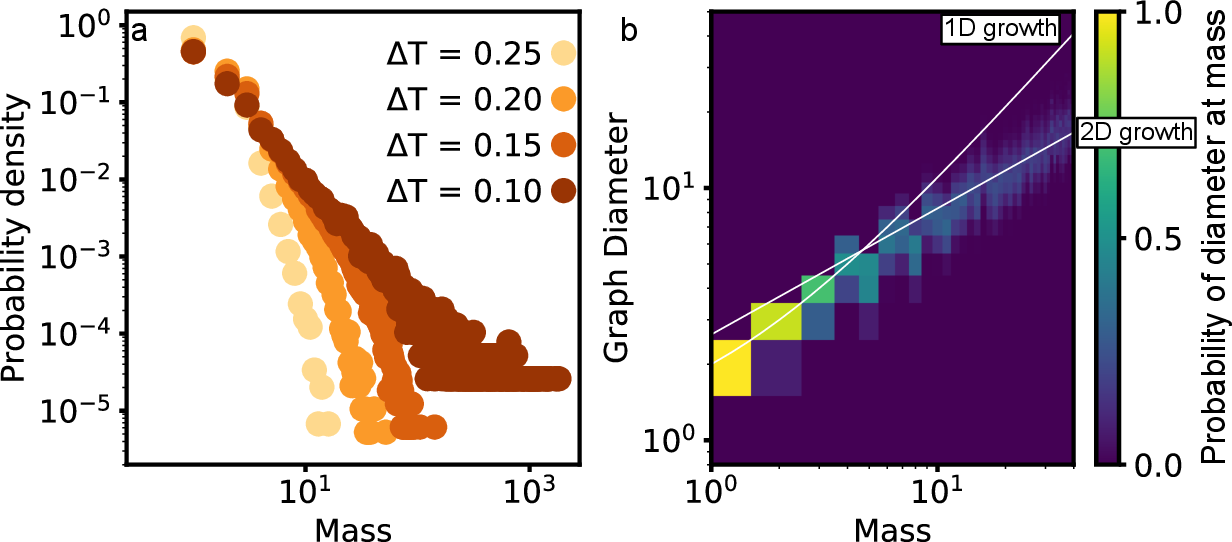
To study the formation of the patchy particle network in more detail, we determine the equilibrium cluster mass distribution at different \(\Delta T\), as shown in Figure 8a. At low attraction, the distribution is cut off at small cluster mass. As the attraction increases (\(\Delta T\) decreases), the mass cut-off moves to the right, indicating formation of larger structures, and eventually, at \(\Delta T = 0.1\) °C, the distribution assumes a power law, indicating percolation of the assembled structure across the plane. This behaviour is qualitatively in line with what we expect for a growing network of patchy particles ⁵³⁾.

We also determine the diameter of the assembled structures, and show a contour plot of diameter frequency as a function of mass in Figure 8b. Initially, at low cluster mass, the diameter increases with a power of 1, indicating growth of linear structures. At higher mass, the diameter increases with the lower power of \(1/2\), indicating the growth of two-dimensional structures.

The transition to the power-law slope \(\frac{1}{2}\) is thus related to the transition from chains to closed clusters: for masses below 4, the ‘cluster’ grows as a linear chain, whose length grows linearly as particles are added. When the clusters grow larger, 2D morphologies become available, like rings, branched chains, and eventually the colloidal graphene lattice. This leads to a transition towards power-law slope of 2, consistent with regular 2D growth. Interestingly, this general scenario is robust, and the evolution of the diameter-mass distribution is largely independent of the density, attraction, and other experimental details of the experiment.

Figure 8: Networking. (a) shows the cluster mass distribution of a structure at four different ΔT. As we increase the attractive strength between patches, the clusters that are formed are typically larger. (b) Probability of finding a graph diameter as a function of mass. Initially, clusters grow linearly, resulting in growth with power 1. As two-dimensional morphologies become available, 2D growth dominates and the power decreases to 1/2.

Normally, we slowly increase the temperature of the system in small, slow steps, waiting at each temperature for four hours, to ensure we observe equilibrium conditions. When we do not do this, and instead heat the system from unattractive (\(\Delta T = 0.40\)°C) to strongly attractive (\(\Delta T = 0.05\)°C), we obtain an amorphous structure, see Figure 9. The formation of such an amorphous structure is in line with our expectations: a very similar process occurs in any other colloidal assembly process, and indeed in atomic systems as well when a fast quench is applied.

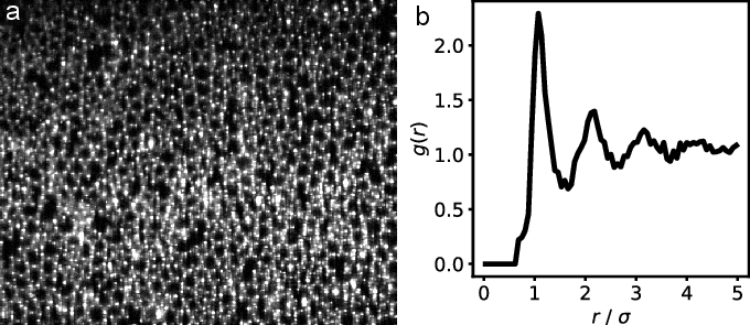
Figure 9a shows an interesting amorphous structure; although there is no clear order, the structure is still very open, and forms rings. The radial distribution function, plotted in panel b of the same Figure, corroborates this observation: there are clearly distinguishable peaks at short range, but these disappear at longer ranges.

Figure 9: A deep quench leads to an amorphous solid. (a) Confocal snapshot of pseudo-trivalent particles frozen into an amorphous solid state after a quenched to high attractive strength. The radial distribution function of this frozen state is show in (b).

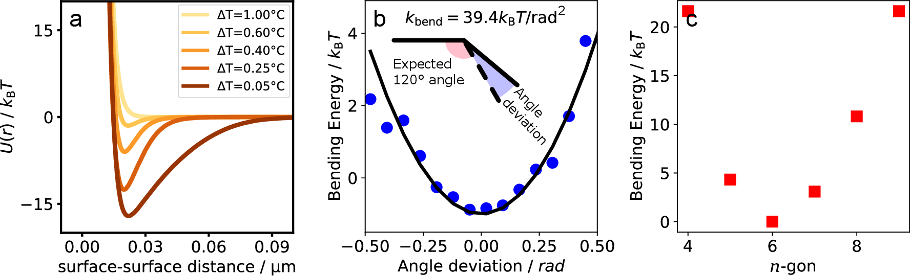
The critical Casimir potential is short ranged, its magnitude and range are set by the temperature offset \(\Delta T = T - T_\mathrm{c}\) to the critical temperature, \(T_\mathrm{c}\). Further factors that determine the magnitude of the potential are the absorption preference of the surfaces (particle patches, glass surface), and the composition of the binary solvent, as detailed in chapter 2⁵⁴⁾. By formulating the critical Casimir potential model presented in  ⁵⁵⁾ for patchy particles and benchmarking it onto our patchy particles as shown in ⁵⁶⁾, we arrive at the attractive potentials shown in Figure 10a. These potentials are valid for ideally opposing patches (no bond bending strain), which is not the case here. Due to the glass-bound patch fixed vertically and the tetragonal patch arrangement, there is always a bonding angle of approximately 60° between the patches in the vertical plane (see Figure 1c). Since this bonding angle is the same for each particle, it equally reduces the bond energy between all particles. Our experiments mostly take place at \(\Delta T =\) 0.05 °C, which means the bonding energy of particles is approximately \(15 k_\mathrm{B}T\).

The bond-bending potential is harder to estimate theoretically, but can be determined from experimental measurements. By following three bonded particles and tracking the fluctuations of their bond angles, we can determine the bending energy by assuming a Boltzmann distribution. The resulting bending energy as a function of angle, determined from the probability distribution of bond angles, is shown in Figure 10b. The shape of this potential can be fitted with a parabola assuming a harmonic potential (Hooke’s law). This leads to a bending stiffness with a force constant of \(39.4 k_\mathrm{B}T \mathrm{rad}^{-2}\).

With this bending stiffness, we can now also determine the energy associated with the bending strain of different \(n\)-membered rings (‘\(n\)-gons’), assuming equal distortion of all bond angles, as shown in Figure 10c. As expected, the bending energy vanishes for hexagons whose inner bond angles match that of the patchy particle. Rings with more or less particles, however, exhibit significant bond bending energy as the inner bond angle deviates from the ideal one. For pentagons and heptagons, the bending energy is only between 4 and 5\(k_\text{B} T\); thus, despite the bending energy cost, pentagons and heptagons are likely to form, which is indeed what we observe.

Figure 10: Bond energies of Patchy Particles. (a) Approximate radial interaction potentials generated by modelled data benchmarked onto experiments (ref. 133). (b) The experimentally determined bending potential (blue circles) between 3 patchy particles at ΔT=0.05°C. The black solid line is a simple Hookean fit, which assumes a simple spring: U_bend=1/2 k_bend θ^2. (c) The bending energy in a regular n-membered ring.

To illustrate the kinetic pathway that leads to the formation of pentagons rather than the equilibrium hexagon motif, we follow a chain of five particles as it closes into a pentagon and tries to open again to form the hexagon at \(\Delta T =\) 0.15°C. We track the particles over time and determine the total energy of the particles in the pentagon as determined from their bond angles, and saturation of bonds. Hence, the energy is determined in the same way as in Figure 4d, that is, we use the sum of the bending energy (using the force constant determined in Figure 10) and the dangling bond energy of the particles involved in the assembly. We also determine the corresponding energy for the formation of a hexagon for comparison. We plot both energy traces as a function of time in Figure 11a. Here, the energy of the ideal 6-membered ring is set to \(0 k_\text{B}T\) as a convenient orientation point.

In Figure 11b we show the expected energy levels of five different structures we observe in the movies: 3 particles bonded in an open chain (labelled \(\text{I}\)), 4 particles bonded in a chain \(\text{II}\)), 5 particles bonded in an open chain (\(\text{III}\)), and the closed 5-particle (pentagon, red) and 6-particle rings (hexagon, blue).

Figure 11: Energy of pentagon and hexagon formation. (a) To illustrate the energetics of a ring closing reaction, we follow two linear chains that will end up as a pentagon (red) and a hexagon (blue) in the assembly process. For each snapshot, we calculate the bending energy and the dangling energy to obtain the total energy and plot it. We set the energy of a closed 6-membered ring to 0, and the other energies relative to that. The solid lines are a guide for the eye. In (b), we show the 5 intermediate structures and their relative energy levels.

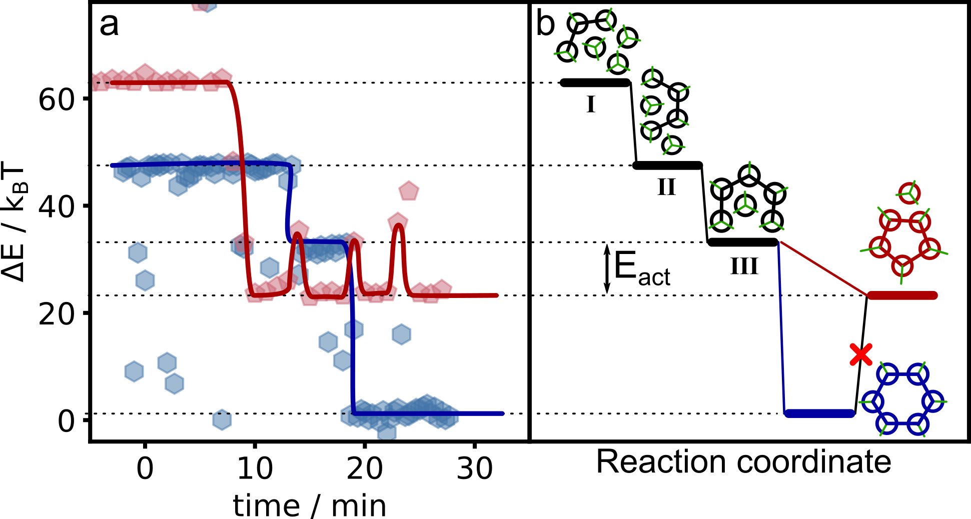
Initially, the three bonded particles have energy of approximately \(62 k_\text{B}T\) (structure \(\mathrm{I}\)). The observed small energy fluctuations are the result of bond-bending due to thermal fluctuations. After 8 minutes, first a fourth particle, and subsequently a fifth particle binds, after which the ring almost immediately closes into a pentagon. The energy drops via the corresponding intermediate values to \(23 k_\text{B}T\), corresponding to the formation of the pentagon. The process is fast, and the intermediate states \(\mathrm{II}\) and \(\mathrm{III}\) are only observed for a single frame each. After the energy drop, the pentagonal ring opens and closes a few times to go back to the open structure \(\mathrm{III}\); however, because no sixth particle is in the correct position to bind, the ring closes before a sixth particle can be incorporated. This way, the pentagon remains metastable.

In the case of hexagon formation, the observation starts with structure $\mathrm{II}$. Now, when the fifth particle binds after 15 min, the structure remains in the open state $\mathrm{III}$; at this point, either a pentagon or a hexagon can form, as is indicated in panel b. This time, another particle is available and binds, and the ring closes into a hexagon after 20 min. This is accompanied by a significant drop in energy to the ground state.

The two examples illustrate in detail the energetic pathway that groups of particles can take to form a ring structure, and are reminiscent of molecular equilibrium reactions. Initially, when structure $\mathrm{III}$ is formed, it is very likely that a pentagon forms shortly after, because this path is energetically favourable though it does not lead to the energetic ground state. Formation of the hexagon requires a 6th particle being available for bonding. Once a pentagon has been formed, an activation energy barrier $E_\mathrm{act} \sim 10k_\mathrm{B}T$ needs to be overcome to open the ring so that another attempt at reacting to a hexagon can occur. If no particle is available, the ring will close again. Several of these attempts are clearly seen in the energy trace of the pentagon (red) in panel a, where the energy jumps to the level of the open ring, but immediately drops back down to that of the closed ring. In this case of an isolated ring, such attempts occur frequently. However, when the ring is embedded in a larger structure, \(E_\mathrm{act}\) can become much bigger due to multiple bonds that need to be broken, to an extent where it is virtually impossible, and the system freezes.

As discussed in the main text, not all defects found in atomic graphene are present in colloidal graphene. In this section, we look at a few common defects in atomic graphene, and calculate how their energies compare to the colloidal analogue, based on the force constants determined in Figure 10a and b. Although these force constants will only yield an approximate energy, they illustrate why certain defects are not present in colloidal graphene where we might expect them.

Figure 12: Schematic structure of several defects in the honeycomb lattice. The different defect types are labelled a-f in the lattice. (a) shows a Stone-Wales defect, caused by a particle pair rotating 90°, resulting in two 5-membered rings and two 7-membered rings. (b) a symmetric single vacancy. One particle is missing from the lattice, which means there are 3 dangling bonds. (c) a monovacancy reconfigured into a 59 defect. This reconfiguration leaves only 1 dangling bond, but does have stretched bonds and strained bond angles. (d) a symmetric divacancy. Two particles are missing from the lattice, resulting in four dangling bonds. (e) a divacancy reconfigured into a 585 defect. This results in the elimination of all dangling bonds, in exchange for strained bond angles and stretched bonds. (f) a divacancy reconfigured into a 555-777 defect. Like the 585 defect, all dangling bonds are removed, but in exchange for strained bond angles and stretched bonds. Red lines indicate strongly deformed bonds, blue dots and dashed lines indicate missing particles and bonds. All these defects' energies of formation are given in the table below.

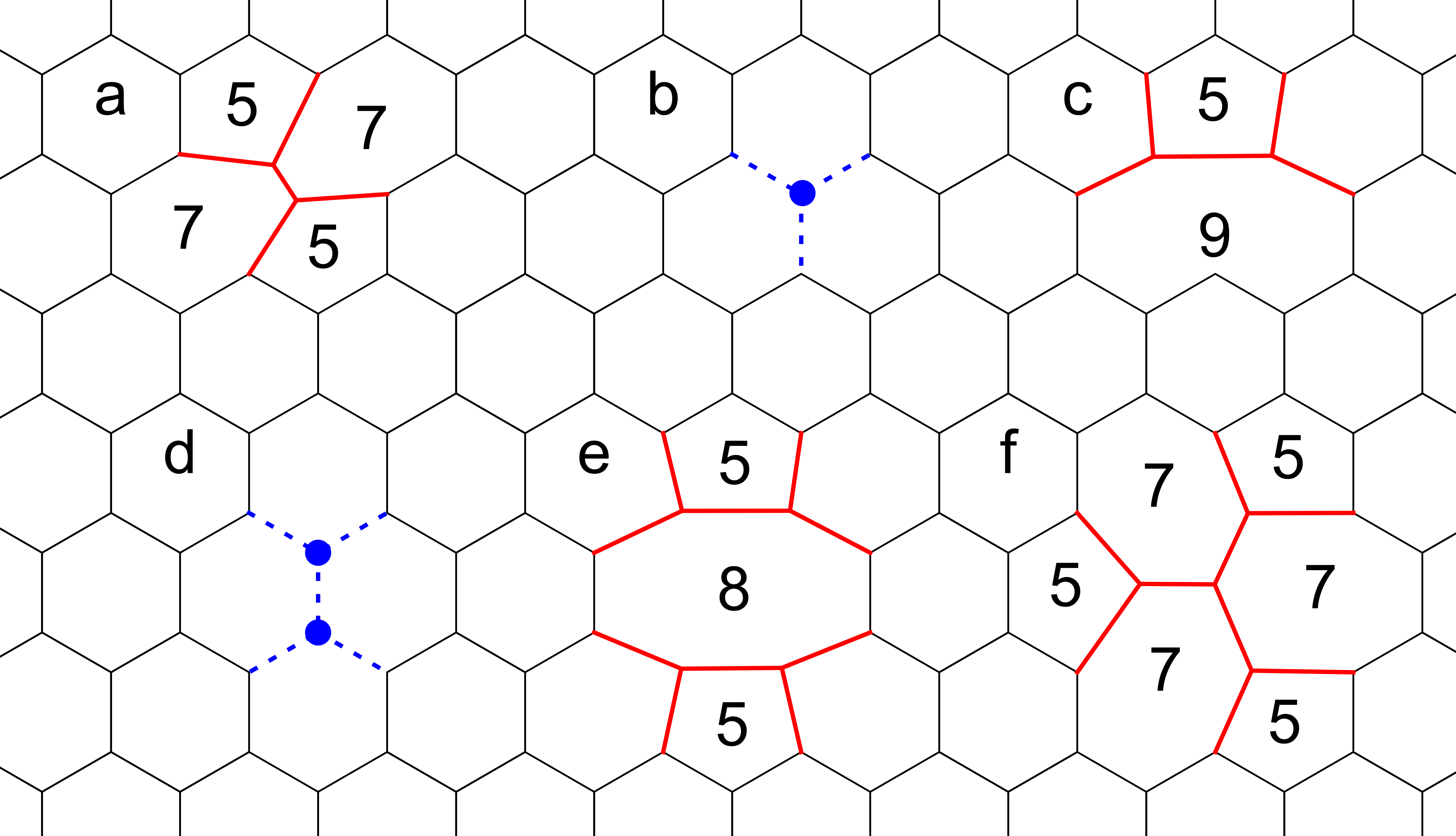
The Stone-Wales defect is a very common type of defect in graphene. It is essentially caused by a particle pair turning 90°C, leading to the formation of two 7-membered and two 5-membered rings, shown schematically in Figure 12 (defect a). The defect is never observed in colloidal graphene. Using the bond bending and stretching energies determined from Figure 10a and b, we determine the energies of formation of the Stone Wales defect in colloidal graphene and compare it to the energy in atomic graphene. We estimate that in colloidal graphene, the defect imposes an energy penalty of \(21 k_\mathrm{b} T\) relative to the regular lattice, which is a very significant penalty. On top of that, to reach this state, a rather large activation energy is necessary to break four particle bonds. Therefore, the Stone-Wales defect is very unfavourable in colloidal graphene, and we do not observe it.

Single vacancies are generally understood to exist in graphene in two distinct ways, the symmetric monovacancy and the 59 (or ‘reconfigured’) monovacancy, shown in Figure 12 (defects b and c)⁵⁷⁾. In atomic graphene, a reconfigured vacancy has only a marginally smaller energy to the symmetric one (only 0.2eV), so there is a small driving force for reconfiguration, see Table 1. The energy difference is small because the crystal lattice around a reconfigured vacancy needs to be deformed, which balances any energy gains due to fewer dangling bonds ⁵⁸⁾. Compared to atomic graphene, the energy penalty of symmetric single vacancies in colloidal graphene is much lower than the penalty for forming the 59 defect, see the table below. This indicates that this defect is unlikely to occur in colloidal graphene, which matches our observations.

Double vacancies exist in the honeycomb lattice in three configurations, the symmetric divacancy (Figure 12, defect d), the 585 divacancy (Figure 12, defect e), and the 555-777 divacancy (Figure 12, defect f). Both the 555-777 and the 585 defects have significantly lower energies compared to the symmetric divacancy in the atomic case, reflected in their ubiquity in defected graphene ⁵⁹⁾. However, in the colloidal case, the energies of the reconfigured configurations are very similar to the symmetric divacancy. In fact, the 585 defect exhibits a slightly lower energy than the symmetric defect. Nevertheless, we do not observe this defect reconfiguring, likely because of the high activation energy such a reconfiguration would need to overcome.

In general, larger vacancies in colloidal graphene have a lower energy penalty for reconfiguration to a state with fewer or no dangling bonds. Activation energies are similarly easier to overcome in larger vacancies. Therefore, large vacancies are expected to reconfigure to some lower energy state, as we can observe in for instance the yellow region of Figure 4a (main text), while small vacancies do not.

Table 1: This table shows the formation energies of several commonly observed defects in atomic graphene. The formation energies of common defects in atomic and colloidal graphene are compared. The energies of colloidal graphene defects have been estimated based on particles positions found in atomic systems, so represent a rough estimate.

Four crystal grains merge into one.

When multiple crystal grains meet during assembly, they will attempt to merge into one bigger grain to minimize the number of dangling bonds. If the two crystals are aligned, the two crystals can be merged easily, resulting in one bigger crystal with no defect. This ‘seamless’ merging has been mentioned in the main text, and we provide an example in Figure 13. Four different crystals meet and form one bigger grain. The red and blue grains merge, and form a new 6-membered ring at their interface. The combination of yellow, green and blue also yield 6-membered rings. Yellow and green are both small structures with no or a few closed rings, and are therefore more flexible with regard to their orientation. The creation of a nice, 6-membered ring is therefore more likely.