Concepts and Methods

When you got right down to it, humans were still just curious monkeys. They still had to poke everything they found with a stick to see what it did.

In published articles, the details of experimental work tend to be swept under the rug somewhat, not because they are unimportant or trivial, but because experiments are, after all, a means to an end. Nonetheless, the experimental process has its own challenges, distinct from the physics we generally try to understand through them, and therefore deserves a closer look. There is a reason the results presented in this thesis are new, and it is not due to freely available low-hanging fruit in the field, nor the lack of imagination from colleagues: it is because the results are very challenging to obtain experimentally. In this chapter, I will try to convey what practical methods I have developed and applied in the past few years, with the sincere hope that it may help any successor(s).

In this thesis, I explore the assembly of diverse structures assembled from simple di-, pseudo-tri-, and tetravalent patchy particles. Recent breakthroughs in particle synthesis have provided strategies to fabricate anisotropic particles, micrometer-size building blocks, which has been a challenge for a long time.

Regular isotropic colloids are often produced using dispersion polymerization ¹⁾. Briefly, in this technique a polymerization reaction takes place in which the polymers are immiscible with the solvent, so that the produced polymers form small precipitates which can grow into colloids. One can vary the exact parameters (solvent, temperature, etc.), but the acting mechanism, the precipitation, will never yield anisotropic particles. Other methods of generating conventional colloids, like emulsion polymerization ²⁾, or the reduction of salts ³⁾, suffer from the same fundamental problem: the nucleation and growth mechanism of these reactions tend to result in spherical particles. Therefore, a fundamentally different synthesis route is needed.

In the past decade or so, synthesis routes to increasingly complex patchy particles have become more commonplace. Of specific interest in this thesis is the particle synthesis developed in the group of Sacanna ⁴⁾. This method, which will be described in detail below, allows for the production of linear dipatch and tetrahedral tetrapatch particles with high specificity and monodispersity. The strategy is to cluster isotropic colloids, which will later form the patches of the particle. Not only the Sacanna-particles described in this thesis are based on this principle, but many successful patchy particle synthesis routes make use of a variation of this principle⁵⁾⁶⁾⁷⁾, although different approaches are also viable ⁸⁾⁹⁾.

The patchy particles used in this thesis are synthesized via colloidal fusion¹⁰⁾ with a modified recipe. Negatively charged polystyrene particles are synthesized by seeded emulsion polymerization using potassium persulfate ($>99.0%$, Sigma-Aldrich) as initiator. After repeated seeded emulsion polymerization, negatively charged PS particles are resuspended into $12.5$mM $\mathrm{NaCl}$ solution. Silicone emulsion droplets are made by hydrolysis and condensation of 3-(trimethoxysilyl) propyl methacrylate (TPM, 98%, Sigma-Aldrich) catalysed by ammonium hydroxide (28 wt.%, Sigma-Aldrich). The droplets are later fluorescently labelled with 3-aminopropyl trimethoxysilane coupled rhodamine-B isothiocyanate. Pluronic F108 triblock copolymer (average Mn 14600, Sigma-Aldrich) is added into the silicone emulsion to a final concentration of 0.05 wt.% to further stabilize the droplets. The F108-TPM emulsion is gently washed by two cycles of centrifugation/resuspension to remove free F108 polymer in emulsion, and later resuspended into 12.5mM $\mathrm{NaCl}$ solution. Tetrahedral colloidal clusters are made by mixing the prepared negatively charged PS particles and F108-TPM droplets at a number ratio around 100:1. To screen the negative charge on both particle surfaces and thus allow for polymer bridging between the two, 12.5mM $\mathrm{NaCl}$ is necessary. These clusters are then separated from excess PS singlets by centrifugation in a glycerol/water mixture (approximately \(22\) wt.% glycerol). The purified clusters are resuspended into aqueous solution containing \(0.05\) wt.% F108 copolymer and \(0.5\) wt.% dodecyl-trimethylammonium bromide (DTAB, $\geq 98\%$, Sigma-Aldrich), to prevent aggregation, and to facilitate core-extrusion during colloidal fusion, respectively. Pure tetrahydrofuran is then added to the cluster suspension to reach a final concentration of \(30%\) \(V_{\mathrm{THF}}/V_{\mathrm{cluster}}\). The fusion is allowed to proceed for 3 minutes before being quenched by deionized water. The resulting patchy particles with liquid patches are then resuspended into deionized water, followed by its polymerization in a 80°C oven for 2 hours. After polymerization, patchy particles typically undergo three centrifugation/resuspension cycles and are transferred back into deionized water for further experiments.

The diameter ratio TPM:PS determines whether a dipatch or tetrapatch particle is obtained - a ratio of 1:3 yields dipatch particles, a ratio of 1:2 yields tetrapatch particles. We have received several batches of di- and tetrapatch particles from the Sacanna group, synthesized by Zhe Gong, each with their own diameter, patch size, and degree of extrusion. The properties of these particles are determined using a variety of techniques (see below), and given in Table 1. Each chapter of this thesis makes use of one or more of these particle batches.

Table 1: Particle stocks. This table shows the most important properties of patchy particle stocks used in this thesis. The patch diameter and patch radius are determined using scanning electron microscopy (SEM), the inter-particle distance is the distance between particles in an assembled structure and is determined using optical microscopy. Values are given with their standard deviations.

Each particle batch is characterized carefully to determine the particle size, patch diameter, and other relevant particle properties. We use three different techniques to characterize particles: scanning electron microscopy (SEM), atomic force microscopy (AFM), and optical microscopy.

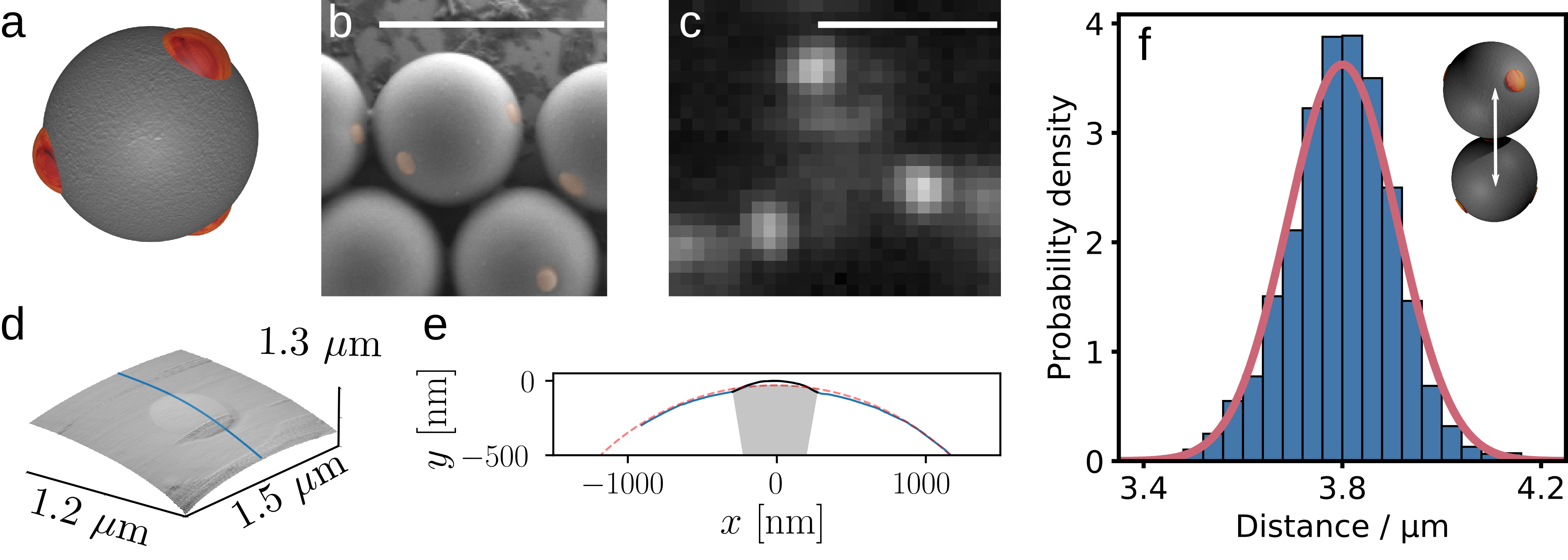
For the SEM measurements, we dilute a particle stock in water, and dry the suspension on a silica surface. Figure 1b shows a typical SEM image of tetrapatch particles. From SEM, we can determine the particle diameter and the patch radius given in Table 1.

AFM can be used for a more accurate estimation of the patch topology. AFM samples are prepared by drying a particle dispersion on a glass microscopy slide. Particles which have a patch oriented upwards are selected for AFM scans. A resulting scan with a clearly visible patch is shown in Figure 1d. By taking a cut through the patch, we obtain the line scan as shown in Figure 1e, which yields the particle and patch radius by simple fitting of the respective curvatures, as well as the patch height and patch radius of curvature.

Finally, effective particle dimensions can be determined directly from optical microscopy images of assembled particles. In an assembled structure, the inter-particle distances of bonded patchy particles should correspond to the effective particle sizes, consisting of the particle diameter, patch height and interaction range. To illustrate this, I perform the analysis for particles of batch A (Table 1). Very good consistency is observed between this measure and AFM/SEM measurements: the distribution of particle-particle distances of assembled particles of batch A is shown in Figure 1f. The mean distance between particle centres is 3.8μm reflecting the SEM-determined particle size (particle diameter \(\sigma= 3.7\)μm plus twice the AFM-determined patch height $2\times48$nm = $96$nm), plus the (short) critical Casimir interaction range, while the standard deviation of $\sigma = 0.11$μm reflects the estimated particle size variation (110nm) and twice the variation of the patch height ($2 \times 5$nm = \(10\)nm). Although this method is rather indirect, it is arguably preferable to AFM or SEM because it measures the relevant parameters in situ. Parameters can be directly related to experiments, while in the case of SEM and AFM measurements, it is not always obvious how the determined parameters correspond to the particles dispersed in solution.

Figure 1: Characterization of patchy particles. (a) Schematic of tetrapatch particle. (b) Scanning electron microscopy image of a tetrahedral patchy particle (batch A in Table 1). The patches are given a false colour. The scalebar indicates 5μm. (c) Confocal image of a tetrahedral patchy particle (batch C in Table 1). The scalebar indicates 2μm. (d) Atomic force microscopy image of a tetrapatch particle (batch A in Table 1). (e) 2D cuttrough of the AFM image along the blue line in (d). The blue line shows the bulk, the black line the patch. The dashed red line is the projected particle diameter σ. Patch diameter, patch height, and patch radius of curvature can be determined from this image. (f) Distribution of inter-particle distances in a structure assembled of particles from batch A in Table 1 (in blue). A normal distribution is fitted to the data (red line), resulting in an average inter-particle distance of 3.80μm with a standard deviation of 0.11μm.

Now that we have discussed the building blocks to assemble, let us discuss the force bringing and keeping assemblies together. Over the years, different methods for colloidal assembly have been developed. At the time of writing, the popular ways of enticing assembly in the lab are DNA-linkers ¹¹⁾, depletion attraction ¹²⁾, or the use of an external force, like a magnetic or electronic field ¹³⁾. However, in our lab, we are specialized in the less common critical Casimir force (CCF) for colloidal assembly ¹⁴⁾. The critical Casimir force is a specific, tunable interaction that arises in binary solvents close to their critical temperature. It results from the confinement of solvent fluctuations between two immersed surfaces, and can be precisely tuned by varying temperature and absorption preference of the confining surfaces.

What does the critical Casimir force offer us that other, more conventional forces for assembly lack? Firstly, the critical Casimir effect is universal: if a binary solvent with an accessible critical point is chosen, interaction between particles will always occur, meaning particles do not need to be made of a specific material to work (like when using magnetic particles). A specific surface is also not necessary; no surface treatment needs to be performed for particles to become attractive (like when using DNA linkers). Secondly, the critical Casimir force can easily be tuned in strength by varying the temperature, giving excellent control over the interaction strength between particles. Finally, by controlling the ratio of the solvents in the binary solvent, the critical Casimir force can be made selective for a specific boundary condition set by surface chemistry. This final point is of critical importance for patch-patch assembly: we can make patches attract only other patches and ignore the bulk, simply by making sure the patch and the bulk have a different affinity for the solvent components.

As a drawback of using the critical Casimir force, we are usually strongly tied to the solvent composition; even small changes can severely influence the behaviour of the system. From a practical perspective, there are experimental designs in which changing the density and refractive index of the solvent is useful or even necessary, specifically when a density match or index match of the solvent to the particles is required. A more application-based problem is the toxicity of the required solvents: the binary solvents typically used to induce critical Casimir forces are all somewhat toxic (they are typically pyridine-derivatives, see below), which excludes practical applications in a larger or commercial setting that requires direct human interaction, like biomedical applications.

In this thesis, we use critical Casimir interactions to assemble patchy colloidal particles. An exhaustive theoretical treatment of the critical Casimir effect is available in literature ¹⁵⁾¹⁶⁾, and only a brief introduction into the basic concepts will be provided here, which should give the reader a solid background to navigate the remainder of this thesis.

The critical Casimir force (CCF) arises in a so called ‘binary solvent’, a solvent consisting of two components. A binary solvent will demix into two separate phases when the demixing line is crossed, see the schematic in Figure 2a. The critical point on this phase diagram, which is situated at a critical temperature \(T_\mathrm{c}\) and a critical composition \(C_\mathrm{c}\), plays a crucial role in the critical Casimir force. When the system approaches the critical point from the one-phase region, phase separation does not take place, but there will be increasing composition fluctuations: locally one of the solvent components has a higher concentration than the other. The correlation length of these fluctuations, $\xi$, diverges as we approach the critical point with $\xi = \xi_{0} \left( \frac{T_\mathrm{c} - T}{T_\mathrm{c}} \right)^{-\nu}$, where $\xi_{0}$ is a system-specific parameter set by molecular pair potentials, and $\nu$ is the universal Ising exponent¹⁷⁾. )) ^18)19)20). Two surfaces close to each other can confine these composition fluctuations, causing an effective attractive force between them: the critical Casimir force ²¹⁾. The exact interaction between surfaces is set by experimental parameters which are fixed for a particular system: the solvent and the geometry and wetting properties of the confining objects. Because the correlation length of the critical fluctuations $\xi$ grows as $T$ approaches $T_\mathrm{c}$, the attractive strength of the CCF grows as well. The latter is only set by $T_\mathrm{c} - T = \Delta T$, the distance of the current temperature to the critical temperature, see Figure 2d.

In this thesis, we typically work at slightly off-critical solvent compositions. Say we approach the coexistence temperature $T_\mathrm{cx}$ at a concentration $C_{2}$, left of $C_\mathrm{c}$ in Figure 2a. At this composition, we are still close to $C_\mathrm{c}$, so composition fluctuations increase as we approach the critical temperature. The fluctuations will predominantly consist of the component which is in shortage in the bulk, e.g., at concentration $C_{2}$ we have a ‘shortage’ of lutidine in the bulk, so any fluctuations are lutidine-rich. This is crucial, because if a surface has a preference for one of the species in the binary mixture, they are sensitive to the composition of the fluctuations. In Figure 2a, left of $C_\mathrm{c}$ there are lutidine-rich fluctuations, which induces attraction between hydrophobic surfaces, while right of $C_\mathrm{c}$ there are water-rich fluctuations, which induces attraction between hydrophilic surfaces.

Figure 2: The critical Casimir effect. (a) The phase diagram of a water-lutidine binary mixture. At temperatures below the critical temperature T_c, there is only one phase, above T_c. the solvent phase separates into a water-rich and a lutidine-rich phase (dark blue region). Close to T_c, there are composition fluctuations. On the left side of C_c, fluctuations are lutidine-rich, and this cause hydrophobic surfaces to attract (green region). On the right side of C_c, fluctuations are water rich, and this cause hydrophilic surfaces to attract (red region). (b) Particle behaviour at different spots in the phase diagram. At spot 1, the critical Casimir force cannot overcome electrostatic repulsion: particles remain dispersed. At spot 2, in the green region, hydrophobic (green) particles attract, while hydrophilic (red) particles remain dispersed. At spot 3, visa versa: hydrophobic particles remain dispersed, while hydrophilic particles assemble. Finally, at spot 4, in the 2-phase region, phase separation occurs and the critical Casimir force is no longer relevant. (c) Assembly of patchy particles with hydrophobic patches and a hydrophilic bulk, in the green region of the phase diagram of panel (a). (d) The inter-particle attraction potential, composed of electrostatic repulsion and critical Casimir attraction, increases as a function of ΔT, the distance to T_c.

Selective particle assembly could thus proceed as follows: consider a mixture of hydrophilic and hydrophobic particles, both with a small electrostatic charge for stabilization and a solvent composition $C_2$, to the left of $C_\mathrm{c}$, along which we slowly increase temperature, lowering $T$, and approaching $T_\mathrm{c}$. Initially, at large $T$, there are only very small composition fluctuations, which cause only minor attraction between particles, not enough to overcome their stabilizing repulsive electrostatic interactions (Figure 2b1). As $T$ decreases, the attractive strength between particles grows, and we reach a point where the hydrophobic particles start aggregating, $T_\mathrm{a}$ (Figure 2b2). Hydrophilic particles do not attract in this situation, and remain suspended. On the other hand, if we had chosen a lutidine fraction right of $C_\mathrm{c}$, such as $C_\mathrm{3}$, hydrophilic particles would assemble, and hydrophobic particles would not (Figure 2b3). In both cases, the attractive strength increases until finally, we cross $T_\mathrm{cx}$ and the binary solvent phase separates, rendering the critical Casimir force irrelevant (Figure 2b4).

Patchy particles combine the properties of the hydrophilic and hydrophobic particles described above. The particles employed here consist of a hydrophilic bulk and hydrophobic patches. This means that by selecting the solvent composition, we determine which part of the particle becomes attractive upon approaching $T_\mathrm{c}$. Typically, we want the patches to be attractive, which means that we choose a composition left of $C_\mathrm{c}$ in Figure 2a, for instance C_\mathrm{2}. When we approach $T_\mathrm{c}$ at this composition, the hydrophobic patches become attractive, while the hydrophilic bulk experiences only negligible attraction. This should lead to patch-to-patch assembly, indicated in Figure 2c. The behaviour can be easily inverted by taking a composition on the other side of $C_\mathrm{c}$, making the bulk attractive and leaving patches neutral.

As discussed above, this thesis will focus on the practical aspect of the critical Casimir effect rather than its theoretical underpinning. Therefore, the next few paragraphs will discuss practical problems, pitfalls and procedures involved in making the critical Casimir force work in real life.

The equipment typically used for temperature control (see section 3.2 below) has excellent relative accuracy: deviation around a set temperature can be kept within a 0.02°C range. However, the absolute temperature will not be accurate at this very fine scale: not only is careful calibration necessary to achieve this precision, but reported and actual temperatures will vary day-to-day due to environmental conditions, like seasonal variation in room temperature and the thermal contact of a sample with its heating elements. Since the strength of the CCF is very sensitive to small changes in $T$ (see for example Figure 10a), we cannot make use of the fluctuating absolute temperature, but must instead rely on an internal temperature calibration: the coexistence temperature $T_\mathrm{cx}$. $T_\mathrm{cx}$ is easily found in experiments (it is the temperature at which phase separation takes place), and temperatures can be defined relative this point. Conveniently, since the coexistence line of the phase diagram is flat close to the critical concentration (see Figure 2a), $T_\mathrm{cx} \approxeq T_\mathrm{c}$ in most experiments, meaning that $T_\mathrm{cx} - T \approxeq T_\mathrm{c} - T = \Delta T$; the distance to $T_\mathrm{cx}$ is directly related to the strength of the critical Casimir forces. This assumption does not hold very close to $T_\mathrm{c}$, but this is rarely the case in practice.

Using $T_\mathrm{cx}$ as internal temperature control also solves another problem: variation between samples and measurements. Even when working extremely carefully, small differences in binary composition, salt concentrations, etc. will exist between individual samples and stocks. All these hard-to-quantify parameters, as well as environmental effects, are reflected in $T_\mathrm{cx}$, which can vary up to a few tenths of a degree between samples. However, the behaviour relative to $T_\mathrm{cx}$ will hardly change, conveniently catching most of these minute variations.

In this thesis, we make use of a binary solvent of 2,6-lutidine (commonly referred to as lutidine) and water. As mentioned, the critical Casimir effect is universal and arises in any binary solvent, however the water-lutidine system has some significant practical advantages. Crucially, the system has a lower critical solution temperature (LCST) just above room temperature at a very convenient temperature of approximately 34 °C ²²⁾. In a binary system with an LCST at or below room temperature, the sample would need to be cooled when not performing experiments, which is very inconvenient. A system with an upper critical solution temperature (UCST), like most binary solvents, is also not ideal: if the UCST is below room temperature, it requires accurate cooling below room temperature, which is more challenging than heating, and if the UCST is above room temperature, the sample would need to be heated when not performing experiments - also not ideal. On top of that, the lutidine-water mixture is well studied, and its phase diagram and critical behaviour, like viscosity and refractive index, have been well known for decades ²³⁾²⁴⁾. Finally, lutidine is a bit less toxic and easier to work with then some of its commonly used alternatives, like 3-picoline and (heavy) water ²⁵⁾²⁶⁾. However, several other binary solvents with suitable properties are available over which the water-lutidine system does not offer significant benefits. Examples include 2-butoxyethanol and water ²⁷⁾²⁸⁾, and 1-propoxy-2-propanol and water ²⁹⁾. Even solvents with micelles can and have been used to induce critical Casimir forces, although micelles will typically also cause depletion interactions as a side effect, making them less convenient ³⁰⁾³¹⁾.

Apart from lutidine, water and particles, a typical sample also contains salt. Salt screens the charges on the particles so that the critical Casimir force can overcome the electrostatic repulsion. Besides suppressing electrostatic interactions, salts can also influence the critical Casimir force: preliminary tests with a few common salts $\mathrm{MgSO}_4$, $\mathrm{KCl}$, and $\mathrm{CaCl}_2$ reveal that magnesium sulfate enhances the attraction contrast between the particle patches and matrix ³²⁾. This is important, because selective patch-to-patch assembly of patchy particles can only take place when there is sufficient contrast between patch and bulk. Ideally, the particle bulk behaves as a hard-sphere particle, while the patches are attractive.

Though only partially understood, ions have been shown to effectively shift the adsorption preference of colloidal particles in binary mixtures, thereby strongly changing their critical Casimir interaction ^{33) 34)}. The underlying reason may be in the special interactions between water and ions, the so-called specific ion effects. These effects are ubiquitous, especially in biochemistry, where it was first remarked upon over a century ago ³⁵⁾. Despite the knowledge of the existence of specific ion effects, its origin is poorly understood, and only empirical descriptions exist, like the famous Hoffmeister series ³⁶⁾³⁷⁾. The origin seems to lie in the different solvation energies surrounding certain ions ³⁸⁾, causing a range of secondary effects: different surface tension and different protein solubility among others.

Another salt-induced effect that could play a role in our particle systems is the solvent preference for individual ions. Some salts are antagonistic: they consist of a hydrophobic and a hydrophilic ion. It is known that the preference of these ions for either component of the binary solvent can influence the phase diagram of water-lutidine significantly ³⁹⁾. In the ‘simple’ magnesium sulfate salt we use, this effect is likely small, but it could play a role.

It is not clear that either specific ion effects or antagonistic salts are at play in increasing patch-to-bulk attraction contrast, but it does illustrate that there is more to salt ions than just their charge, especially in a system close to the critical point of demixing, where such effects may be amplified. Careful screening and selection of the salt in a system is required to optimize the patch-to-patch attraction.

To investigate the properties of particle bulk and patches separately, and find the optimal conditions for the patchy particle assembly, we first focus on the assembly behaviour of the two particle components of the patchy particle, polystyrene (PS) and 3-(trimethoxysilyl) propyl methacrylate (TPM). We use the precursor PS spheres of the colloidal fusion synthesis of particle batch A (Table 1), and TPM droplets polymerized under the same conditions as the patches. This results in solid TPM particles of diameter \(\sigma = 1\)μm that have the same surface properties as patches in the final composite patchy particle.

We vary the composition and salt concentration of the binary solvent to determine the optimal selective TPM-TPM (and thus patch-to-patch) attraction. For this purpose, TPM and PS particles are dispersed in binary mixtures of varying lutidine concentration for microscopic characterization. Samples are imaged while the temperature is slowly increased towards $T_\mathrm{c}$ using a temperature-controlled stage (see section 3.2). An oil-immersion objective with 63x magnification is used for bright-field imaging. By increasing the temperature slowly we identify the aggregation temperature $T_\mathrm{a}$, at which clear cluster formation occurs (as shown in Figure 3a) and the coexistence temperature $T_\mathrm{cx}$, at which bubbles form. From this, we construct aggregation lines with respect to the solvent phase-separation line as a function of lutidine concentration as shown in Figure 3b.

The aggregation lines in Figure 3b show that without $\mathrm{MgSO_4}$, PS particles (blue line) and TPM particles (red line) aggregate stronger for lutidine concentrations right of the critical composition, meaning that they both show the same water-philic affinity and thus no selective patch-to-patch attraction. However, by adding 0.5 mM of magnesium sulfate, the aggregation behaviour of TPM particles changes completely: a strong critical Casimir attraction is observed to the left of the critical composition, green line in Figure 3b. This indicates that the adsorption preference of TPM switches to lutidine-philic when adding \(\), while the aggregation temperature of PS particles is little affected and remains water-philic as can be seen from the snapshots that show cluster formation of PS still happens on the right side of the critical temperature, Figure 3a (bottom right). Using the aggregation curves, we pinpoint a sweet spot where only TPM particles are expected to attract (small violet-shaded region in Figure 3b).

Figure 3: Enhancing the contrast for critical Casimir patch-to-patch binding. (a) Bright field images showing aggregation contrast of PS particles (big dots) and TPM particles (small dots). The former make the bulk, the latter the patch of the composite patchy particle. Clockwise, starting top left, conditions are: c_lut=28%vol, MgSO_4=0mm; c_lut=32%vol, MgSO_4=0mM; c_lut=25%vol, MgSO_4=0.5 mM; and c_lut=32%vol, MgSO_4=0.5 mM. Scale bar is 3μm. (b) Aggregation diagram showing the shifted aggregation lines of TPM without salt (red diamonds), with MgSO_4=0.5mM (green circles), and PS without salt (blue squares). Black continuous line shows theoretical coexistence temperature of the binary mixture close to the critical point. Coloured stars and pentagons indicate corresponding measurement condition of (a). Purple dotted line indicates a good lutidine concentration for patchy assembly (25%vol).

After determining the best solvent composition, all our experiments are performed in the region where we obtain the strongest selective patch-to-patch attraction: we use an optimal lutidine concentration $c_{\mathrm{lut}} = 25\%\mathrm{vol.}$, with 1 mM $mathrm{MgSO_4}$ that shows the largest range of TPM-TPM (and thus path-to-patch) attraction while PS is not attractive.

The vast majority of the experiments performed in the context of this thesis relies on optical microscopy to observe the assembly process and resulting structure - specifically laser scanning confocal microscopy. All experiments are performed under accurate temperature control, as to control the strength of the critical Casimir force. Microscopy can yield rich and insightful information on a local level - one can literally see what happens at the microscopic level, but the technique is less suited for bulk behaviour and averages, because it only catches a relatively small area of the sample at a time. Scattering techniques (SAXS, SANS, SLS, etc.) are more suitable for bulk characterization, and are therefore also the more traditional techniques for probing colloidal length scales. However, microscopy is the method of choice for the study of patchy particle assemblies. Not only do patchy particles typically have interesting local behaviour, but, as highlighted in chapter 1, patchy particle assemblies typically are very small, rendering scattering experiments meaningless.

A widely-recognized problem with microscopy data analysis is the risk of (unconscious) bias. Therefore, it is of particular importance to go from images to usable data in a reproducible and objective way. In this section, I will set out to explain the process of preparing the sample, briefly describe the microscopy setup, and finally describe the analysis of the microscopy data, specifically with regard to (patchy) particle tracking.

The patchy particles are stored dispersed in water with a small amount of F108 copolymer as stabilizer (< 0.05%wt). To prepare a sample stock, particles are transferred to the binary solvent by washing them at least 4 times in the desired binary mixture. This mixture can be stored in small centrifugation tubes for a few weeks. To prepare a sample for microscopy, a small amount of the sample is injected into a glass capillary (Vitrotubes, Rectangle Boro Tubing 0.20 mm) and sealed with teflon grease (Krytox GPL-205), see Figure 4.

In some cases, we use hydrophobic silanized glass capillaries. The hydrophobic treatment for capillaries is a simple gas silanization reaction. The capillaries are cleaned thoroughly using a piranha treatment, or alternatively using Hellmanex III and plasma treatment. Capillaries are then placed in a vacuum desiccator together with approx. 1 ml of hexamethyldisilazane (HMDS) ($\geq 99.0$, Sigma-Aldrich). Pressure is lowered to below 200 mbar using a pump, and kept low for at least 2 hours. The capillaries are then baked in an oven at 120 °C for circa 1 hour. Microscopy samples can then be prepared as usual with these capillaries ⁴⁰⁾⁴¹⁾.

Figure 4: Sample preparation. After a particle dispersion with the right concentration has been prepared, the dispersion is injected into capillaries to be able to observe the sample under a microscope. To prepare a sample, (a) teflon grease is injected into one end of a capillary. (b) The particle dispersion is then very carefully injected into the capillary from the non-sealed opening using a 10 μL micropipette. (c) The open end of the capillary is now also injected with teflon grease, closing off the mixture from the environment. We now have a capillary ready for microscopy.

Samples that are properly sealed with teflon grease will remain stable for approximately 1 month. If the ends are properly sealed with an extra layer of glue (Norland Optical Adhesive, nr. 81), samples can be stable without significant change in function for over a year.

Figure 5: The microscope and its temperature control. An overview of the microscopy setup is shown in (a). The waterbath controlling the temperature is labelled 1. The coil heating the objective is labelled 2, and is highlighted in (b). The sample holder is labelled 3, and is highlighted in (c). In (d), the heating system is shown schematically, with the water flow between elements indicated, adapted from ref 123.

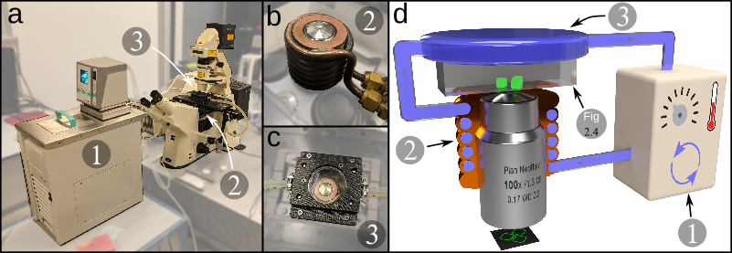
All samples are imaged on a Zeiss Axiovert 200M inverted optical microscope, either in bright field, fluorescence (532nm laser) or confocal (LSM 5 Live line-scanning confocal microscope module with 532nm laser) mode. The microscope is equipped with a well-controlled temperature stage in combination with an objective heating element, as fine temperature control is indispensable to make use of the critical Casimir force. Relative temperature accuracy far below a tenth of a degree, needed to have meaningful control over patch-to-patch attraction in our system, is achieved using a home-built closed loop water system.

The temperature control is based on water flowing through the components of the microscope that are in contact with the sample, see Figure 5: the sample stage on which the sample is mounted, and the objective, which can act as a heat sink by proximity or direct contact (in case of an air or oil objective respectively). Accurate control of the water temperature thus leads to accurate control over the sample temperature. We use a Julabo D25 ME waterbath to pump temperature-controlled water through the sample stage and objective. The sample stage consists of a glass cell trough which water can flow. The transparent glass stage allows bright-field microscopy to be performed with the illumination from the top, a significant advantage over available commercial solutions. The objective is heated by the temperature-controlled water flowing through a brass tube coiled around it.

This setup allows for a relative temperature accuracy of about 0.01 °C with minimal temperature gradients while performing microscopy. This is easily verified by looking at the data gathered in this thesis, much of which would be impossible without very accurate and stable temperature control.

To extract useful data from the microscopy images, we track all particles in the field of view, meaning we determine their \(x\), \(y\), and possibly \(z\) coordinates. In fluorescence microscopy, fluorescent colloidal particles manifest as Gaussian peaks in intensity. The most common way to locate these peaks is by using the algorithm proposed by Crocker and Grier in the 90s ⁴²⁾. Not only does the algorithm find fluorescent features, it finds them with sub-pixel accuracy by fitting to a Gaussian distribution instead of simply finding the centre ⁴³⁾. This means that, even though a pixel size is typically not much smaller than the feature of interest, locations can be determined with an accuracy of up to \(0.2%\) of the feature radius.

Recently, machine learning has started to become more common in scientific image analysis. Especially complicated environments with a lot of background and noise (e.g., biological samples) benefit from improvements in noise reduction and detection optimization ⁴⁴⁾⁴⁵⁾. However, to my knowledge, machine learning algorithms are currently not matured enough to outperform the classical Crocker-and-Grier algorithm in relatively simple colloidal systems.

The specific software we use for particle tracking is Trackpy, a modern Python implementation of the Crocker-and-Grier algorithm ⁴⁶⁾. After loading an image and optimizing parameters, it can accurately determine patch locations in two or three dimensions. However, in this thesis, simply finding the bright spots in an image is only the first step in determining particle locations. Patchy particles are synthesized such that the patches are fluorescent (see section 1 above). A tetrameric patchy particle will thus not have one bright spot, but four, each of which are at a different \(x\), \(y\), and \(z\)-position. On top of that, if particles are bonded patch-to-patch we observe just one fluorescent dot which represents two bonded patches, belonging to different particles. To accurately track particle centre, orientation, and bonding, different algorithms were designed and implemented, depending on the details of the system and the information available.

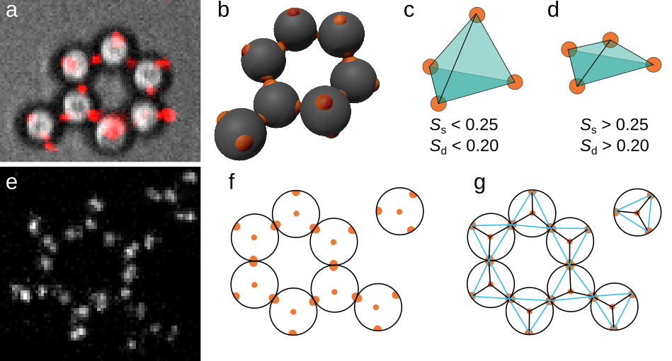
In chapter 3, we discuss the formation of clusters of five particles, each bonded with two other particles. Accurate three-dimensional tracking of the particles is achieved by overlaying bright field and confocal microscopy channels, shown in Figure 6a. Figure 6b shows the full three-dimensional representation of the ring. We determine the particle location and orientation in five steps:

1. Determine the two-dimensional centre of particles from the bright-field channel.
2. Determine the three-dimensional centre fluorescent patches from an entire confocal image stack.
3. Using the estimated particle and patch centres from steps 1 and 2, determine which patches (potentially) belong to the same particle.
4. Draw a tetrahedron for all possible combinations of 4 patches that could belong to the same particle, as shown in Figures 6c&d.
5. Determine the angular tetrahedrality order parameter $S_\mathrm{g}$ and the distance order parameter $S_\mathrm{d}$:

$$ S_\mathrm{g} = \sum_{i=1}^4 \sum_{j=1,j \neq i}^4\left( \mathbf{r}_i \cdot \mathbf{r}_j + \frac{1}{3} \right)^2 $$ $$ S_\mathrm{d} = \sum_{i=1}^4 \frac{ \left(d_i - \overline{d}\right)^2 }{\overline{d}^2}$$ with $i$ and \\(j\\) patch indices, \\(\mathbf{r}\\) the unit vector pointing from the centre of the 4 patches to a patch, and \\(d\\) the length of \\(\mathbf{r}\\). If these order parameters are below a threshold (typically \\(S_\mathrm{g} < 0.25\\), \\(S_\mathrm{d}<0.20\\)), the group of patches forms a regular tetrahedron of the right size; we assume these are patches that make up a particle, see Figure 6c. If the threshold is not reached, we are observing a false positive, see Figure 6d.

We have thus determined 4 patches belonging to the same particle, the average location of which is the particle centre. We can determine whether particles are bonded by simply checking which particles share a patch.

Figure 6: Overview of tracking procedures developed in this thesis. (a) Representative microscopy image of particles as taken in [[en:research:phdthesis:ch3|chapter 3]], where we use confocal images (in red) superimposed onto bright-field microscope image. Note that because we project a 3D image onto a 2D image, most particles seem to have only 3 patches per particles, while they have 4. (b) 3D representation of situation shown in (a). (c) A group of 4 patches belonging to the same particle, forming a regular tetrahedron, which has an S_g and S_d below the threshold value. (d) A group of 4 fluorescent features, forming an irregular tetrahedron, which has an S_g and S_d above the threshold value. One or more of the features is likely a false positive. (e) Representative z-projected confocal microscopy image of particles as taken in [[en:research:phdthesis:ch4|chapter 4]]. (f) Representation of situation shown in (e). Particles have a black outline, patches are shown in orange. The central patch is slightly out of focus, and will thus be less bright in (e). (g) The network formed by connecting all patches within a particle radius of each other. Regular triangles, and thus the groups of connected outer patches are shown in cyan.

Unfortunately, the double channel approach is not always feasible because it requires double channel microscopy: the switching between channels makes the measurement slow. Therefore, in chapter 4 & chapter 5, we employ a slightly different approach. In this situation, particles are all at the same height, with one patch bound to the surface and the other three available for bonding. Although this particular conformation is not strictly necessary for this tracking approach to succeed, it does simplify tracking significantly. In Figure 6e, a typical microscopy image is shown, with in Figure 6f a schematic representation of the situation. Each particle has one central patch in the centre of the particle, and 3 patches at the edge of the particle. To find particle positions, we perform the following actions:

1. Determine the location of each fluorescent patch.
2. Find all other patches within approximately one particle radius, by using a kd-tree (implemented in SciPy) ⁴⁷⁾, and connect those into a network.
3. Find all triangles in the resulting network (Figure 6g).
4. For each triangle, we determine the mean edge length and the variation of this value. We only select triangles where the mean edge length \(d\) is close to the expected value based on radius \(r\) (\(d = r\)), and where the edge length variation is small. This means we effectively select the blue triangles in Figure 6g.

We are left with a triangle with 3 vertices corresponding to the outer patches. In the centre of the triangle is the patch bound to the surface. Particle bonds are easily determined by checking which patches are shared between particles.