Phases of surface-confined trivalent particles
Chaos is merely order waiting to be deciphered.
In the previous Chapter, we have studied the assembly of pseudo-trivalent patchy particles into colloidal graphene. Here, we further elucidate the complex phase behaviour of these particles: besides the honeycomb phase, we observe an amorphous network phase and a triangular phase. Structural analysis is performed on the three condensed phases, revealing their shared structural motifs. Using a combined experimental and numerical simulations approach, we elucidate the origins of these phases and construct the phase diagram of this system. Using appropriate order parameters, we accurately determine coexistence lines in the phase diagram. Our results reveal the rich phase behaviour of the relatively simple patchy particle system, and open the door to a further joined simulation and experimental exploration of the full patchy-particle phase space.
1. Introduction
Colloidal particles are an ideal system for studying the assembly of complex materials. Despite their apparent simplicity, colloidal particles can assemble into complex structures, sometimes even mimicking atomic materials, while still being easily studied using simple scattering or microscopy methods 1). Modern synthesis methods can go far beyond the classic isotropic colloidal sphere, endowing particles with special properties like specific particle shape and valency 2)3)4). A subfield of colloidal assembly that has grown especially prominent over the past decade is the study of so-called patchy particles. A patchy particle is a colloid decorated with patches of a different material than the bulk; the patches are typically used to induce specific attraction to other patches, and thus to steer the assembly towards specific phases. Simulations and theoretical studies have revealed a wealth of structures that even relatively simple patch geometries can assemble into 5)6)7).
In the past, probing patchy particle assembly was performed largely through simulations, due to the challenge of synthesizing these particles bottom-up and introducing and controlling the anisotropic interactions. However, recent advances in colloid chemistry and new experimental strategies have made possible the production of more complex geometries of patchy particles and the study of their assembly 8)9). Experimental realization of reversible patch-patch bonding is still challenging, but opens the door to many complex structures, analogues of atomic compounds and beyond 10)11)12). One way to realize selective patch-patch attraction of tunable magnitude is through critical Casimir interactions that depend on the solvent affinity of the particle surfaces 13)14). The critical Casimir force arises in binary solvents close to their critical point when the confinement of solvent fluctuations between the particle surfaces causes an effective attractive force on the order of the thermal energy, \(kT\), tunable by the temperature offset \(\Delta T\) from the solvent critical point, \(T_\text{c}\).
It is tempting to think of the assembly of patchy particles as simple binaries: either patches are not attractive and do not assemble, or patches are attractive, and assembly starts. Reality is fortunately much more interesting; simulations reveal that patchy particles often have rich phase behaviour, and equilibrium structures do not only depend on particle geometry, but also on patch attractive strength and particle density 15)16)17). Although hints of complex phase behaviour are sometimes reported in experimental work 18), it has never been the primary object of study.
In this work, we experimentally explore the phase diagram of surface-confined, pseudo-trivalent particles that interact via critical Casimir forces. The critical Casimir force allows us to finely adjust the attraction between particles, enabling easy access to the full range of the phase diagram. We observe the formation of three structurally distinct condensed phases: the honeycomb lattice, an amorphous network, and the so-called triangular phase. The honeycomb lattice has been studied comprehensively in chapter 4, but the less intuitive amorphous and triangular phases have never been observed experimentally. We elucidate the basic morphological motifs of the three condensed phases and reveal how the phases are structurally related. Finally, we use the bonding state and typical lattice distances as structural order parameters to pinpoint the phase transition between the phases. Our results reveal that simple surface-confined trivalent particles display a surprisingly complex phase diagram, highlighting the rich phase behaviour even very simple patchy particles can display. Our results open the door to a larger effort towards a joined simulation and experimental exploration of the full patchy-particle phase space.
2. Methods
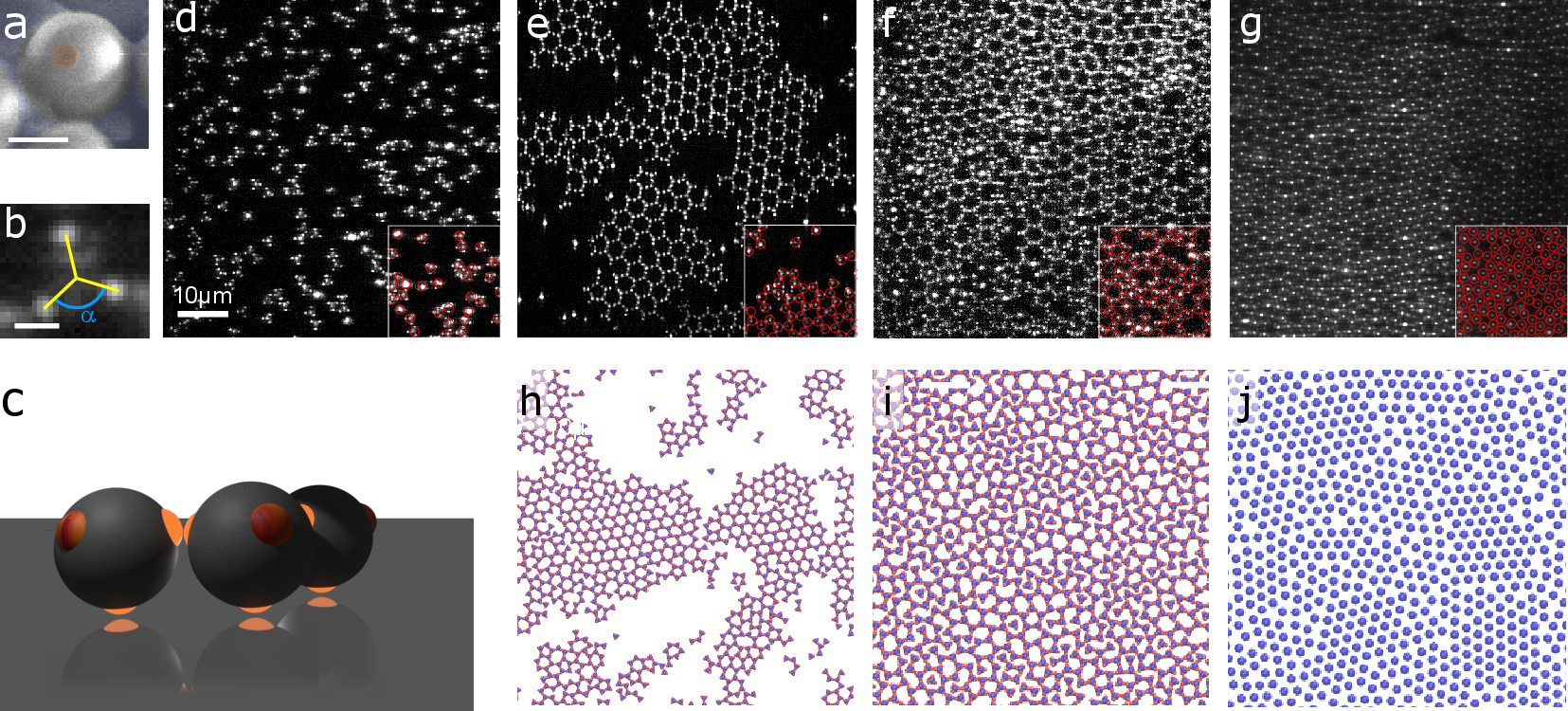
In this chapter, we make use of a system similar to the one described in chapter 4. We use particle batch C from Table 1: tetrapatch particles consisting of a polystyrene (PS) bulk and fluorescently labelled 3-(trimethoxysilyl)propyl methacrylate (TPM) patches, with a diameter of 2.0 μm and a patch diameter of 0.2 μm, see Figure 1a&b 19). We suspend the particles in a binary mixture of lutidine and water close to its critical point to induce an effective patch-patch attraction. The confinement of solvent fluctuations between the particle surfaces then causes attractive critical Casimir interactions, tunable by the temperature offset \(\Delta T\) from the solvent critical point, \(T_\mathrm{c}\), see chapter 2.
We use a binary mixture of lutidine and water with lutidine volume fraction \(c_\mathrm{L} = 0.25\) close to the critical volume fraction \(c_\mathrm{c} = 0.27\) 20), and solvent demixing temperature \(T_\text{cx} =\) 34.12 °C, and add 1 mM of \(\mathrm{MgSO_4}\) to screen the particles’ electrostatic repulsion and enhance the lutidine adsorption of the hydrophobic patches (see chapter 2. The suspension is injected into a glass capillary with hydrophobically treated walls to which the particles become adsorbed via one of their patches at \(\Delta T \leq\) 0.7 °C. The resulting pseudo-trivalent particles diffuse freely along the surface (see chapter 4, section 5.2, until approximately \(\Delta T \leq\) 0.45 °C, when the free patches start attracting each other noticeably.
To study the formation of phases, we let the sample assemble by slowly approaching \(T_\text{c}\) in steps of 0.01 K or larger (up to 0.05 K), starting from \(\Delta T =\) 0.65 °C. The sample is prepared with a particle density gradient by slightly tilting the sample, so it is easy to observe a range of different area coverages \(\eta\) at a constant \(\Delta T\), see section 5.1. We take confocal microscopy images at several points in the sample and track both the particles’ centre of mass and fluorescent patches to determine the bond angles with their neighbours (for tracking details, see chapter 2. While 1 of the 4 patches is bonded to the glass, the other 3 patches can participate in bonding and are at approximately the same height (see Figure 1c). By focussing at different heights, we can accurately determine the horizontal position of the particle centre (from the glass-bound patch) and the bonds between particles (from the bonding patches).
Simulations
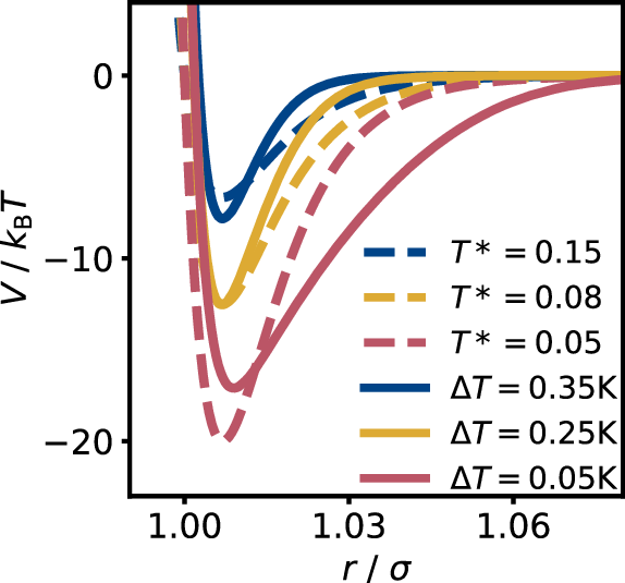
In parallel with experiments, we also perform Monte Carlo (MC) simulations, to aid the mapping of the phase space. The interaction between particles is set by a generalized Lennard-Jones (LJ) repulsive core and an attractive tail modulated by an angle dependent function, which is a reasonable model for our patchy particle system 21)22). Further simulation details are given in Appendix below. Simulations are performed at a range of different reduced temperatures (\(T^*\)) and surface coverages. In section 5.3, we compare the inter-particle potentials at several \(\Delta T\) and \(T^*\) to be able to directly compare experiments and simulations at similar attractive strength.
3. Results and Discussion
At low patch-patch interaction strength (high \(\Delta T\)) and low density (approx. \(\eta < 0.5\)), particle patches interact only weakly, resulting in a two-dimensional colloidal fluid, see Figure 1d. We measure the diffusion constant of the particles, see chapter 4, section 5.2, showing that colloids can freely diffuse laterally over the surface. At higher patch-patch interaction strength, starting from \(\Delta T \approx \) 0.38K, particles form a honeycomb lattice in equilibrium with a dilute fluid phase, see Figure 1e. In the lattice, each particle binds three other particles at 120° angle with respect to each other resulting in the typical repeating 6-membered rings motif of the honeycomb lattice. The honeycomb lattice is common in nature and engineering at all length scales due to its extraordinary mechanical and electronic properties. Famous examples include graphene, which is formed by the two-dimensional assembly of trivalent atoms 23)24).
At higher densities, more exotic equilibrium structures emerge. Around an area fraction of \(\eta = 0.55\), an amorphous network is observed, Figure 1f. This network is characterized by a wide distribution of ring sizes, in which particles exhibit non-ideal bond angles, slightly above or below 120°. The open nature of the honeycomb lattice is preserved, but the order is lost: the rings do not periodically tile the surface like in the honeycomb lattice, but fill the area seemingly without long-range order. At yet higher density, at an area fraction of approximately \(\eta > 0.6\), the particles pack tightly in the triangular phase, Figure 1g. The triangular lattice consists of a honeycomb structure in which each honeycomb cell is occupied by an additional particle. Particles are ordered in a dense hexagonal close packing (hcp), but still bind to neighbours within the lattice due to their attractive patches.
Simulation snapshots of the system at similar density and attractive strength as the experimental snapshots are shown in Figure 1h-j. The simulations seem to capture our experimental results very well: simulated and experimental snapshots display remarkably similar structures; the three condensed phases are formed both in experiment and simulation.
3.1. The Phase Diagram
To gain a more complete understanding of our system, we construct a density-temperature phase diagram based on our experiments in Figure 2a, and simulations in Figure 2b. The fluid phase is indicated in grey, the honeycomb-fluid coexistence in yellow, the amorphous network phase in blue and the amorphous-triangular coexistence phase in red. Each point in the diagram represents an observation.
In experiments, the fluid phase (microscopy snapshot overlaid with particle orientations shown in Figure 2c), is present at high \(\Delta T\) (low interaction strength) and low density, and consists of freely diffusing, mostly unbound particles. The fluid-to-honeycomb transition occurs upon increasing interaction strength (decreasing \(\Delta T\)) as indicated by arrows 3 to 6, or when increasing density, along arrows 1 & 2. A microscopy snapshot of the fluid-honeycomb coexistence is shown in Figure 2d.
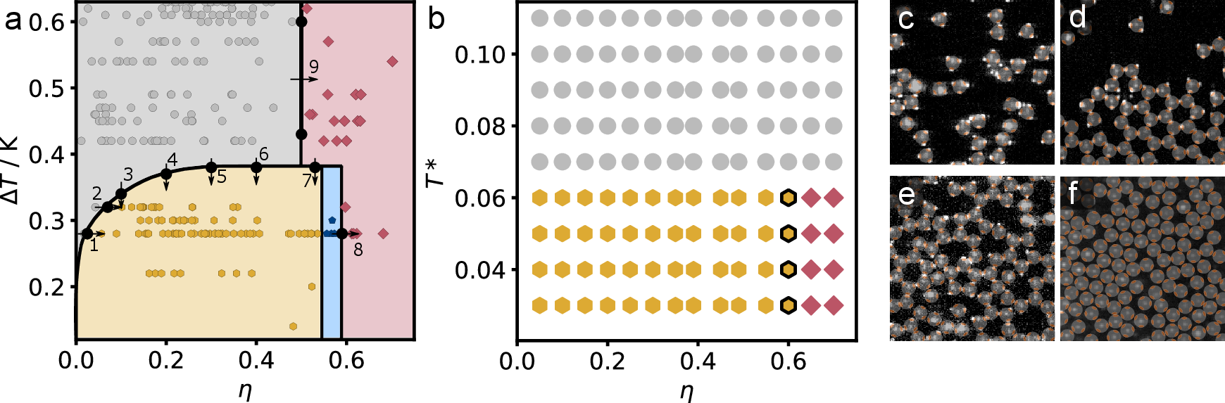
In experiments, a phase transition from fluid-honeycomb coexistence to the amorphous phase takes place at surface coverage \(\eta = 0.53\). The amorphous phase, Figure 2e, leaves part of the open honeycomb structure intact, but packs particles at a higher density by introducing different ring sizes. This results in a structure which is slightly density than the honeycomb lattice, and contains only few unsaturated patches. Due to its open structure, the honeycomb lattice has a maximum packing fraction \(\eta \approx 0.60\), beyond which the lattice simply cannot accommodate more particles. The amorphous network on the other hand can accommodate higher particle densities, but pays an energy penalty for bending bonds out of their equilibrium angles to from non-ideal ring sizes.
As density increases further, another phase transition is observed in experiments: along arrow \(8\) in Figure 2a, a transition from the amorphous network to a coexistence of amorphous and triangular phases takes place. The triangular lattice is shown in Figure 2f, and consists of particles assembled in a hexagonal close-packed (hcp) structure, such that as many patch-patch bonds as possible are formed. The triangular phase is essentially just the honeycomb lattice with additional particles placed in the centre of each hexagon. This leads to at least 20% of patches being unsaturated in equilibrium, which makes this phase energetically unfavourable at lower densities.
The simulations phase diagram, Figure 2b, is mostly in agreement with the experimental phase diagram: the fluid, fluid-honeycomb and amorphous-triangular phases are all present at approximately the same attractive strength and density (see section 5.3). Unfortunately, the density-induced fluid to fluid-honeycomb coexistence transition cannot be verified in simulations, due to difficulties in equilibrating the MC simulations at these very low densities.
In simulations, we observe a pure honeycomb lattice, a feature not found in experiments. This is not surprising: due to the short range of the critical Casimir force (in the order of \(0.01 \sigma\), section 5.3), the pure honeycomb region is expected to be extremely narrow and easily missed, and kinetic effects may quickly lead to the amorphous phase.
Furthermore, a pure amorphous phase is not observed in simulations. Instead, there is an immediate transition from honeycomb to amorphous-triangular coexistence. The amorphous and triangular phases can accommodate a high particle density at the expense of bending and dangling bonding energy penalties, respectively. This means that the bond flexibility of the patchy particle determines what structure is energetically more favourable: if the particle’s bond bending energy penalty is relatively minor compared to the dangling bond energy penalty, we expect the amorphous phase to take up an extended region in phase space. If, on the other hand, bond bending carries a large energy penalty due to e.g. narrow patches, we expect to see a gradual transition from honeycomb to triangular, without an intermediate amorphous phase 25). In our experimental system, the bond bending energy cost is estimated to be on the order of \(40 kT\mathrm{rad}^{-2}\) (assuming spring-like bending, see chapter 4, section 5.6, leading to a small energy penalty to the formation of penta- and heptagons. A difference in this value between experiments and simulations may thus explain why experiments show a narrow amorphous region, while simulations do not show an amorphous region at all.
In experiments, the triangular phase is encountered at low interaction strength (high \(\Delta T\)), contrary to the other condensed phases, and contrary to what simulations show. As the patches are only weakly attractive at such high \(T\), our particles act somewhat like isotropic colloids. We hypothesize that the crystallization along arrow \(9\) in Figure 2a is akin to simple hard-sphere crystallization under high pressures. The transition at \(\eta_9 \) is lower than expected based on purely hard-sphere interactions, and is not observed in simulations, but reasonable if we assume there is likely some bulk-bulk attraction 26).
3.2. Structural Analysis
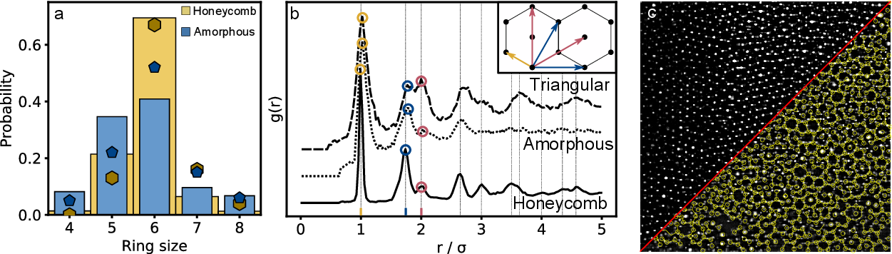
To further elucidate the nature of the amorphous and triangular phases and their relation to the honeycomb lattice, we analyse their structures. Important structural motifs are the rings, the sizes of which are characteristic of the phases: they are strictly 6-membered in the honeycomb lattice, and more broadly distributed in the amorphous phase. The ring size distribution of both phases are shown in Figure 3a, bars indicate experimental measurements, dots indicate simulation results. As expected, both the experimentally obtained and simulated honeycomb phase consists primarily of 6-membered rings, but also shows a small fraction of 5- and 7-membered rings. While the perfect honeycomb lattice would purely consist of only hexagons, the experimental and simulated lattices display defects, mostly at grain boundaries (see chapter 4), leading to deviations from perfect hexagons. Nevertheless, the amorphous network phase displays a much broader distribution of ring sizes, indicating that this phase consists of a variety of motifs in its bulk, including large fractions of 5- and 7- membered rings. This broad ring size distribution is a hallmark of two-dimensional trivalent particle networks: similar distributions have been found in amorphous silica and the theoretical triangle network, even though the bond details (bending and stretching strain) are very different from our case 27). The ring-size distributions from experiments, compared to the ones from simulations reveal an interesting kinetic effect: the number of 5-membered rings in experiments is significantly larger, while the number of 7-membered rings is smaller than in simulations. The origin of this difference may lie in kinetic effects, favouring smaller ring sizes in experiments, and in the different effective patch sizes of experiments versus simulations.
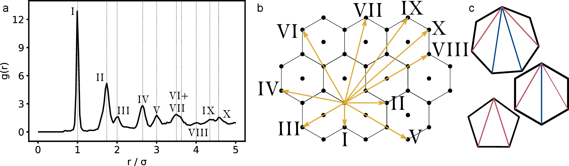
We can further compare the experimental amorphous and honeycomb phases via the pair correlation function \(g(r)\), plotted in Figure 3b. Surprisingly, even after the expected nearest-neighbour peak at \(1 \sigma\) (1 particle diameter), the \(g(r)\) of the two phases is remarkably similar: all visible peaks seem to coincide, indicating similar short-range structure. For the amorphous phase, however, peaks diminish after a few particle radii, while for the honeycomb phase, peaks are still well-defined even at long distances. The short-range similarity of the amorphous and honeycomb radial distribution functions is a direct result of their very similar basic structural motifs. Both phases consist of rings related to the particles’ vacancy: hexagons in the honeycomb case, a mix of mainly penta-, hexa-, and heptagons in the amorphous case. These rings share similar typical internal distances, leading to a very similar short-range radial distribution function (see section 5.5). The amorphous \(g(r)\) decorrelates at larger distances because each shell of rings introduces a diverging number of ring size combinations and associated characteristic distances. Although some ring combinations are preferred, see section 5.6, the decorrelation is inevitable, and consistent with the lack of long-range order of the network. These effects are in line with other observations of amorphous networks consisting of trivalent subunits, and have been observed at length scales spanning from atomic to macroscopic 28).
In contrast to the honeycomb and amorphous phases, the triangular phase is characterized by hexagonal close packing, giving rise to a dense network of patch-patch bonds within this packing. These two layers of organization are exemplified in the microscopic image in Figure 3c. The glass-bound patches (equivalent to particle centres) in the top-left clearly show the hcp lattice of the phase. The bottom-right of Figure 3c highlights the network of bonds between particles overlaid onto the image. Combined, both halves of Figure 3c reveal the complex internal structure of the triangular phase at low \(T\) that is not revealed by simple particle locations.
The close vicinity of the triangular to the honeycomb lattice, with each honeycomb cell occupied by another particle, is reflected in the \(g(r)\) (Figure 3b): the peak positions of the triangular lattice largely coincide with those of the honeycomb lattice, but the peak intensities are different: for instance, the peak at \(1.74 \sigma\), corresponding to a particle in the ring, and the peak at \(2.00\), corresponding to both particle in a ring and the central particle of a ring, have different relative heights. In the honeycomb lattice, the peak at \(2.00 \sigma\) is smaller than the one at \(1.74 \sigma\), reflecting the absence of centre particles in the open honeycomb lattice compared to the triangular lattice: in the latter, both distances are equally likely, while in the honeycomb case, the \(2.00 \sigma\) distance only occurs half as often, see inset of Figure 3b. The intensity ratio \(R\) of the two peaks thus characterizes open and closed phases: a ratio below \(1\) indicates an open structure (the honeycomb and amorphous phases), while a ratio above \(1\) corresponds to the closed triangular phase, and a ratio close or equal to \(1\) indicates that neither peak is present, signalling a disordered fluid phase.
3.3. Order Parameters
Based on the structural properties discussed, we can now define order parameters to construct the coexistence lines between the phases in the experimental phase diagram. To do so, we follow the main structural changes along isobars and isotherms, and use structural order parameters to pinpoint the phase transition lines.
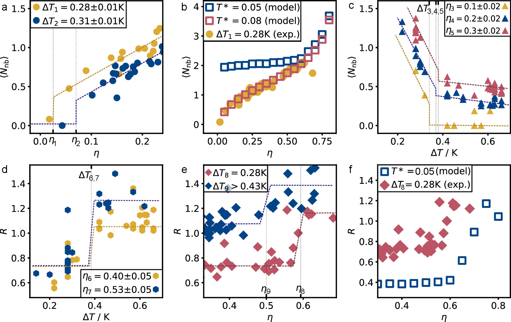
The fluid phase is characterized by a low number of bonded neighbours, therefore, the fluid-honeycomb phase transition along arrows \(1\) to \(5\) in Figure 2a is easily determined using the mean number of neighbours \(\langle N_\mathrm{nb} \rangle\) of a particle. We define nearest neighbours as those particles with centres found within \(1.1\sigma\) of the particle under consideration. In Figure 4a, we show \(\langle N_\mathrm{nb} \rangle\) as a function of surface coverage \(\eta\) at two different interaction strengths. In both cases, \(\langle N_\mathrm{nb} \rangle\) jumps from \(0\) to a non-zero value, signalling the transition from a low-density fluid phase to fluid-honeycomb coexistence. After this point is reached, \(\langle N_\mathrm{nb} \rangle\) increases monotonically along the \(T_1\) and \(T_2\) isotherms, indicating the growth of the honeycomb lattice at the expense of the fluid phase. In Figure 4b, we follow the same order parameter for the simulations at two constant attractive strengths. The behaviour is strikingly similar to that in the experiment: the evolution of \(\langle N_\mathrm{nb} \rangle\) at \(T^{*}=0.08\) and \(\Delta T=\) 0.28 K almost perfectly overlap, as expected from their similar attractive strength (section 5.3). Although the discontinuity is not observed in simulations due to problems with equilibrating the system at low densities, the similarity between simulation and experiment suggest a fluid-fluid transition as well. In contrast, at higher interactive strength, \(T^{*} = 0.05\) - equivalent to approx. \(20kT\), \(\langle N_\mathrm{nb} \rangle\) plateaus at low density; the fluid-honeycomb coexistence phase extends all the way to low density.
We also explore the isobaric path at constant density and increasing attraction, by plotting the experimentally observed \(\langle N_\mathrm{nb} \rangle\) as a function of \(\Delta T\) at three different volume fractions in Figure 4c. In the fluid phase, at low attraction (high \(\Delta T\)), \(\langle N_\mathrm{nb} \rangle\) is low. When the attraction increases, \(\langle N_\mathrm{nb} \rangle\) jumps and increases strongly, signalling the transition from the fluid phase to honeycomb-fluid coexistence. Still, only at the lowest density \(\eta_3 = 0.1\), the fluid phase shows vanishing $\langle N_\mathrm{nb} \rangle$. At higher volume fractions \(\eta_4 = 0.2\) and \(\eta_5 = 0.3\), \(N// \) no longer vanishes; the reason is twofold: firstly, particles in the fluid can bond transiently; bonds form, but break up before particles get close to forming the honeycomb lattice. Secondly, at higher densities, particles are statistically more likely to be within the nearest-neighbour range without being bonded. These tendencies lead to slight continuous increase of $\langle N_\mathrm{nb} \rangle$ before reaching the true phase transition. \(\langle N_\mathrm{nb} \rangle\) is therefore not the ideal order parameter to identify the phases at higher densities. Instead, we can make use of the characteristic distances of the condensed phases of \(1.74\sigma\) and \(2.00\sigma\). Specifically, the characteristic height ratio \(R\) of the \(g(r)\) peaks at \(1.74\sigma\) and \(2.00\sigma\) can be used as an order parameter indicative of the phase transitions.
Because of these properties, \(R\) is a suitable order parameter for characterizing the transition from fluid to amorphous or honeycomb phases, specifically at high density, e.g. paths \(6\) & \(7\) in Figure 2a, whose \(R\) values are shown as a function of \(\Delta T\) in Figure 4d. The transition from fluid to honeycomb lattice is signalled by a jump of \(R\) from below \(1\) in the open lattice to approximately \(1\) in the fluid phase, placing the phase transition at \(\Delta T_6 \approx 0.35\). The isobar along \(\eta_7 = 0.53\) acts differently: instead of \(R\) jumping to \(1\), \(R\) becomes larger than \(1\), indicating a transition from an open structure to the triangular phase, as shown in the phase diagram in Figure 2a.
\(R\) is also a suitable order parameter to detect the transition from the triangular to the amorphous phase, arrow \(8\) & \(9\) in Figure 2a. We follow \(R\) as a function of \(\eta\) at \(T_8 =\) 0.28K in Figure 4e. The clear jump at \(\eta_8 = 0.58\) indicates the phase transition from the open amorphous lattice to the triangular lattice. The simulations show a similar transition from an open to a closed structure in Figure 4f. The transition occurs at a slightly higher density compared to the experiments, which is expected given the somewhat shifted phase diagram of the simulations. The difference in magnitude of \(R\) between simulation and experiment is probably due to the inherent noise present in the experimental data, leading to \(R\) values closer to \(R=1\).
Finally, we also use the peak ratio \(R\) to follow the density-induced transition from unordered fluid to triangular phase in the absence of strong patch-patch attraction (arrow \(9\) in Figure 2a). By plotting \(R\) as a function of \(\) for \(T_{9} >\) 0.43 K in Figure 4e. Although \(R\) is by no means the ideal parameter to signal this transition 29), a jump does clearly occur at around \(\eta_{9} = 0.5\), indicating a transition to an ordered phase.
4. Conclusion
By utilizing the excellent control over patch-patch attraction offered by the critical Casimir force, we experimentally explore the pressure-interaction phase diagram of pseudo-trivalent colloidal particles adsorbed at a substrate. This relatively simple system displays a surprisingly rich phase behaviour, not only assembling into the honeycomb lattice, but also into an amorphous network and a triangular phase at increasing particle density. Combining our experiments with simulations, we find that the three condensed phases are structurally closely related, and a delicate balance between bending and bonding energies determine their interconversion. By following order parameters along isobars and isotherms, we construct the phase diagram of the system.
The exploration of the complex phase diagram illustrates the increasingly advanced control over patchy particle assembly, and opens the door to experimental investigation of the full phase space of the assembly of patchy particles with different valencies. The surprisingly rich assembly behaviour found in this simple patchy particle system hints at a wealth of interesting behaviours in more complex systems; there is a huge phase space to explore, while varying parameters such as density, attractive strength, particle geometry, and system dimensionality.
5. Appendix
5.1. Sample Preparation and Measurements
Tetrapatch particles (diameter of 2.0 μm, patch diameter of approx. 0.5 μm, batch C in table 1 of chapter 2, see also chapter 4, sections 5.3 & 5.6) are dispersed in the regular binary solvent of 25% 2,6-lutidine (>99%, Sigma Aldrich) and 75% milliQ water with 1 mM \(\mathrm{MgSO_4}\), as described in chapter 2. The particles are washed several times in the water-lutidine mixture. The resulting particle dispersion is injected into a silanized hydrophobic glass capillary and sealed with teflon grease (for full preparation see chapter 2).
5.1.1. Confocal Microscopy and Particle Tracking
Particles are left to sediment to the bottom of the sample at room temperature before measurements. We tilt the sample slightly during sedimentation, so a small density gradient is present in the sample. We then heat the sample to 33.45 °C ($Delta T \approx 0.65$°C), which causes one of the particle patches to attach to the sample wall. For heating, we use a well-controlled temperature stage in combination with an objective heating element.
In an experiment, we typically heat a sample to a certain \(\Delta T\) below the phase separation temperature of the lutidine-water mixture, inducing critical Casimir attraction between patches. The structures then grow by two-dimensional diffusion in the plane. No mixing is necessary. After several hours of equilibration, we investigate the structures using a 100x oil-immersion objective.
We image the assembled structures using confocal microscope image stacks, sometimes alternating with bright field images. We track the particle locations via the network-based approach described in chapter 2. The highest density samples (i.e, the triangular phase) could not be tracked using this technique: there were too many outer patches to consistently identify bonds. However, particle centres could still be accurately determined. The bonds shown in Figure 3c are determined by naked eye.
5.2. Simulation Details
5.2.1. The Potential
The interaction between particles is described by a generalized Lennard-Jones (LJ) repulsive core and an attractive tail modulated by an angular dependent function 30)31):
$$ V_{ij}(\mathbf{r}_{ij},\mathbf{\Omega}_i,\mathbf{\Omega}_j) = $$
$$ V_{\mathrm{LJ}}^\prime(r_{ij}) \text{ , if } r_{ij} < \sigma_{\mathrm{LJ}}^{\prime} $$
$$ V_{\mathrm{LJ}}^\prime(r_{ij}) V_{\mathrm{ang}}(\mathbf{\hat{r}}_{ij}, \mathbf{\Omega}_i,\mathbf{\Omega}_j) \text{ , if } r\_{ij} \geq \sigma\_{\mathrm{LJ}}^{\prime}$$
where \(_{ij}\) is the inter-particle vector, \(\alpha\) and \(\beta\) are patches on particles \(i\) and \(j\), respectively, \(\mathbf{\Omega}_i\) is the orientation of particle \(i\), \(V_{\mathrm{LJ}}^\prime(r)\) is a cut-and-shifted \(m-n\) LJ potential and $\sigma_{\mathrm{LJ}}^{\prime}$ corresponds to the distance at which $V_{\mathrm{LJ}}^\prime$ passes through zero:
$$ V_{\mathrm{LJ}}^\prime (r_{ij}) = \frac{n}{n-m} \left(\frac{n}{m} \right)^{\frac{m}{n-m}} \epsilon_{LJ} \left( \left(\frac{\sigma_{LJ}}{r_{ij}}\right)^n - \left(\frac{\sigma_{LJ}}{r_{ij}}\right)^m\right) $$
The exponents of the generalized-LJ model are assigned large values, in particular 200-100, to obtain a short ranged model mimicking that found in experiments of colloidal particles. The cut-off distance is set to \(r_\mathrm{cut}=1.10\,\sigma_\mathrm{LJ}\), at which the energy is rather small (-0.0029 ϵ).
The angular modulation term \(V_\mathrm{ang}\) is a measure of how directly the patches α and β point at each other, and is given by
$$ V\_\mathrm{ang}(\mathbf{\hat{r}}\_{ij},\mathbf{\Omega}\_i,\mathbf{\Omega}\_j) = \exp \left( -\frac{\theta\_{\alpha ij}^{2}}{2\sigma\_{\mathrm{ang}}^{2}} \right) \exp \left( -\frac{\theta\_{\beta ji}^{2}}{2\sigma\_{\mathrm{ang}}^{2}} \right) ,$$
\(\theta_{\alpha_{ij}}\) is the angle between the patch vector \(\mathbf{\hat{P}}\_{i}^{\alpha}\), representing the patch α, and $\mathbf{\hat{r}}\_{ij}$. Each particle has four patches distributed tetrahedrally on the particle surface. \(\sigma\_\mathrm{ang}\) is a measure of the angular width of the patch. In this study, the angular width is set to \(\sigma\_\mathrm{ang}\)=0.52 radians.
The patches interact also with the bottom surface through the same interaction potential (see definition of $V_{ij}$ above). The difference is that now the distance between the particle and the surface is given by the \(z\)-coordinate of the particle position vector, and the angular term depends only on the Gaussian of the angle of the interacting patch with the normal to the surface. The interaction strength between two particles is set to unity, \(\epsilon\_{LJ}=1\), and that between a particle and the bottom surface is set to \(\epsilon_s=4\epsilon_{LJ}\). We use \(\sigma_\mathrm{LJ}\) as the unit of length, and the LJ well depth \(\varepsilon_\mathrm{LJ}\) as the unit of energy. Temperatures are given in reduced form:
$$ T^*=k\_B T/\varepsilon\_\mathrm{LJ}. $$
Besides these interactions, to mimic the experimental conditions, particles were also subject to a gravitational potential: \(u\_{\mathrm{grav}}(z)=\frac{z}{l\_{\mathrm{grav}}}k\_\mathrm{B}T\) where \(l_{\mathrm{grav}}\) is the gravitational length, whose value was estimated from the relation \(l_{\mathrm{grav}}=k_\mathrm{B}T/\Delta \rho V_\mathrm{c} g\), where \(\Delta \rho\) is the density difference between the colloids and the solvent, \(V_\mathrm{c}\) is the volume of the colloidal particles and \(g\) is the gravitational constant. Here, we took \(l_{\mathrm{grav}}=0.5865\sigma_\mathrm{LJ}\). Note, however, that the effect of this term once the particles are deposited on the surface is small, because the strength of the wall with the particles' patches is stronger.
5.2.2. Simulations
We use Metropolis Monte Carlo to simulate the patchy-particle systems in the canonical ensemble (NVT). The simulations are performed in an orthorhombic box with \(N=900\) colloidal particles. Periodic boundary conditions are applied along the \(x\) and \(y\) axes. Several lengths of the simulation box along the \(x\) and \(y\), \(L_x\) and \(L_y\), are used to cover surface packing fractions, \(\eta=N\pi/L_x/L_y/4\), between 0.001 and 0.85. In order to minimize the incommensurability of the assembled honey-comb and triangular lattices with the simulation box, we set \(L_x=2/\sqrt{3}L_y\). \(L_z\) is initially set to \(L_z=100\sigma_\mathrm{LJ}\). Particles are initially distributed randomly in the simulation box. The system is then allowed to evolve until all the particles sediment and bind to the bottom surface. Using this state as the initial configuration, simulations are then performed at different temperatures. To improve the sampling, besides normal MC moves, aggregation volume moves (AVB) 32) are also performed. The acceptance probability of the MC moves is set to 50-70%. Typically, the MC simulations consist of 100 million MC cycles, where one cycle is defined as \(N\) attempts to translate or to rotate a particle. At the lower temperatures, simulations need to be twice or three times longer to get well converged results.
5.3. Comparing Simulations and Experiments
The reduced temperature \(T^{*}\) sets the interaction strength between particles in simulations, while the distance to the critical temperature \(\Delta T = T - T_\mathrm{c}\) sets the interaction strength in experiments. Unfortunately, relating these two parameter is non-trivial, which limits direct comparison of simulation and experimental results. To nevertheless make a comparison, we plot the inter-patch potentials in simulations and experiment in Figure 5. Simulated potentials result from the Lennard-Jones potential of the previous section, while the Casimir potential is generated by formulating the critical Casimir potential model presented in 33) for patchy particles and benchmarking it onto our patchy particles as shown in 34). We select values of \(\Delta T\) and \(T^{*}\) which result in approximately the same potentials, so that we can estimate at which temperatures similar behaviour is expected. Figure 4b of the main text shows that this approach is effective: the average number of neighbours \(\langle N_\mathrm{nb} \rangle\) as a function of area coverage \(\eta\) in experiments and simulations almost perfectly overlap for \(\Delta T =\) 0.28K and \(T^* = 0.08\), in agreement with their matching potentials in Figure 5.
5.4. Order Parameter R
When our system transitions from an open structure (like a honeycomb lattice or amorphous network) to a closed lattice (the triangular lattice), the systems’ radial distribution undergoes a small but significant change, as illustrated in Figure 3b. The most obvious change occurs at the \(2\sigma\) peak, which is significantly bigger in the triangular phase due to the particle occupying each hexagonal ring. Therefore, we can use the ratio between this peak and the unchanged peak at \(1.74\sigma\) to follow the transition from open to closed structure; we define the ratio between the two peaks:
$$ R = \frac{\int_{1.6\sigma}^{1.9\sigma} g(r) ~\mathrm{d}r}{\int_{1.9\sigma}^{2.1\sigma} g(r) ~\mathrm{d}r} \mathrm{.} $$
This ratio \(R\) has a value below \(1\) in the case of an open structure (the honeycomb and amorphous phases), while a value above \(1\) corresponds to the closed triangular phase, and a value close or equal to \(1\) when neither peak is present, signalling an unordered fluid phase. We use this ratio as order parameter to determine coexistence points between two phases in Figure 4.
5.5. Radial Distribution Peaks
Figure 3b shows the radial distribution function of the honeycomb, triangular and amorphous phases. As we discuss, the typical distances revealed by the radial distribution function of these three condensed phases overlap due to their shared structural motifs. In Figure 6a, we show the radial distribution function of the honeycomb lattice without normalization, with each characteristic distance indicated. In Figure 6b, the corresponding distance is indicated in the honeycomb or triangular lattice. Figure 6c highlights the small difference in internal distances of a 5-, 6-, and 7-membered ring: the two possible distances within a ring, indicated with red and blue are very similar in all three ring types.
5.6. Particle Neighbourhood
In this chapter we have briefly discussed that the amorphous phase shows some local order, but little long range order, highlighted by the radial distribution function shown in Figure 3a, where peaks die away only at longer ranges. Here, we further examine the short-to-medium range order of the amorphous phase by studying the local ring neighbourhood. We find all particle rings in a sample, and determine the probability to find an \(n\)-membered ring as neighbour to an \(m\)-membered ring, see Figure 7a-c. In the honeycomb phase (shown in yellow), 5-, 6-, and 7-membered rings are all most likely to have a neighbouring 6-membered ring. However, it is clear that 5-membered rings are much more likely to be next to a 7-membered ring instead of another 5-membered ring and visa versa. This is in line with the fact that neighbouring 5- and 7-membered rings experience significantly less bonding strain, see Figure 2b: a ‘scar’ of 5- and 7-membered rings is a typical defect seen in assemblies of trivalent, surface-confined building blocks because it is geometrically relatively stable, see chapter 435).
In the amorphous case (shown in blue), the distribution is much more ambivalent: All ring sizes have nearly equal probability of being next to any other ring. This is hardly surprising considering the random packing of these many-sized rings.
A related metric is the probability of ring triplets combinations, given in Figure 7d: the probability of finding 3 rings clustered together, see the inset drawings. In the honeycomb case (blue), the (6,6,6) triplet is by far the most common, as we would expect in this lattice built of hexagons. Other significant fractions include (5,6,7), a typical defect element (see chapter 4 (5,6,6), and (6,6,7). In the amorphous case (yellow), the triplet probability is much more broadly distributed. However, there are still clear preferences, clearly signalling that the amorphous phase is still somewhat ordered over ‘medium’ distances. This matches similar observations in other trivalent amorphous networks, like amorphous silica 36).
